Array constants have been part of Excel for years. One of my early encounters with them was using CHOOSE to rearrange columns so VLOOKUP could look to its left. A useful trick, certainly, but array constants have plenty to offer beyond older lookup formulas.
In today’s dynamic array Excel, they are more useful than ever. A small collection of values inside curly braces can help a formula sort by several columns, split text using multiple delimiters, extract several pieces of a reference, or test a list of conditions.
And this is not just about the newest functions. Good old MID, OR and SUM can benefit too.
You can work through these examples with the practice workbook.
What You'll Learn
- Array constants supply several fixed values to a formula argument using curly braces.
- Corresponding arrays let SORT and MID apply multiple instructions within one formula.
- Lists of criteria simplify status checks and totals across multiple categories.
Table of Contents
- What Is an Array Constant in Excel?
- 1. Sort by Multiple Columns with SORT
- 2. Split Text Using Multiple Delimiters with TEXTSPLIT
- 3. Extract Several Parts of a Reference with One MID Formula
- 4. Test a List of Statuses with IF and OR
- 5. Sum Multiple Criteria with SUMIFS and SUM
- A Small Excel Skill with Plenty of Uses
What Is an Array Constant in Excel?
An array constant is a fixed collection of values written directly into a formula, enclosed in curly braces. Instead of supplying one value to an argument, you supply several.
For example, {4,5} contains two numbers. The array {"East","West"} contains two text values, each enclosed in double quotation marks.
The important question is what the receiving function does with those values. It might use them as column numbers, delimiters, starting positions or criteria. The braces look the same, but their role depends on where you put them.
In the formulas below, commas separate values across columns. That horizontal arrangement is particularly useful when returning several extracted fields side by side. Microsoft’s guide to array formulas provides additional background on working with arrays in Excel.
1. Sort by Multiple Columns with SORT
Sorting by more than one column is hardly unusual. You might want the most important issues first, with the oldest issues appearing first within each priority level.
Our source table, tblIssues, contains issue details, a priority, a reported date and a status. Priority 3 is the most important. FILTER returns only the incomplete issues, and DROP removes the final Status column from the result:
=DROP(FILTER(tblIssues,tblIssues[Status]="Incomplete"),,-1)That gives us the outstanding issues, but we also need them in a useful order.
Start with a single sort column
Wrapping the result in SORT lets us sort by the fifth column, Date Reported, in ascending order:
=SORT(
    DROP(FILTER(tblIssues,tblIssues[Status]="Incomplete"),,-1),
    5,
    1
)
Here, 5 identifies the column to sort, and 1 means ascending. The earliest dates come first.
A quick formula-writing tip: Alt + Enter inserts a line break while editing a formula, making nested functions easier to read.
Use corresponding arrays for multiple sort levels
Now suppose priority must take, well, priority. We want:
- Priority, column 4: descending, so priority 3 comes first.
- Date Reported, column 5: ascending, so older issues come first within each priority.
Replace the individual sort arguments with array constants:
=SORT(
    DROP(FILTER(tblIssues,tblIssues[Status]="Incomplete"),,-1),
    {4,5},
    {-1,1}
)
The two arrays correspond by position. Column 4 pairs with -1, meaning descending. Column 5 pairs with 1, meaning ascending.
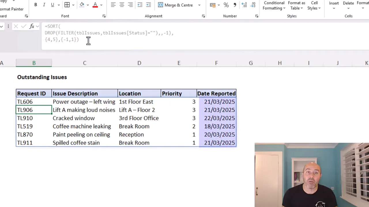
The result places the priority 3 issues at the top. Within that group, 21 March appears before 22 March. One SORT function handles both levels because we have supplied two column numbers and two matching sort orders.
2. Split Text Using Multiple Delimiters with TEXTSPLIT
TEXTSPLIT is another excellent use for array constants. Rather than splitting text at only one character, we can give it a list of delimiters.
Consider a URL containing a coupon code between an equals sign and an ampersand. For a URL in cell A2, the formula is:
=INDEX(TEXTSPLIT(A2,{"=","&"}),1,2)There are two parts to this:
TEXTSPLIT(A2,{"=","&"})splits the URL at either an equals sign or an ampersand.INDEX(...,1,2)returns the second element from the resulting row.
In this URL layout, that second element is the coupon code. The array constant lets TEXTSPLIT recognise both boundaries without needing separate splitting formulas.
The URL structure matters. This formula takes the second piece, so it suits the example where the coupon code follows the first equals sign. It is not searching for a coupon parameter wherever it might appear.
For more examples of this function, see my TEXTSPLIT tutorial.
3. Extract Several Parts of a Reference with One MID Formula
Array constants are not reserved for modern functions. MID has been around for a long time, and it can perform several extractions in one formula.
Suppose a billing reference contains these fixed-width fields:
- A two-character region code, starting at position 1.
- A four-digit billing period, starting at position 3.
- A six-digit document number, starting at position 7.
We could write three separate formulas. Or we could give MID three starting positions and three corresponding character counts.
For one reference in B2:
=MID(B2,{1,3,7},{2,4,6})The matching pairs tell MID exactly what to extract:
- Start at
1and extract2characters for the region. - Start at
3and extract4characters for the billing period. - Start at
7and extract6characters for the document number.
In dynamic array Excel, those three results spill into adjacent columns. We can also provide a vertical range of billing references to process several rows at once:
=MID(B2:B20,{1,3,7},{2,4,6})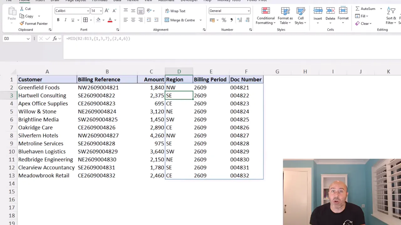
This is the same principle as the SORT example: values in corresponding positions work together. The first starting position uses the first character count, the second uses the second, and so on.
The source reference can also be made dynamic. That is a separate technique, covered in my dot operator tutorial. The useful point here is that one familiar text function can return several fields simply by accepting arrays of instructions.
4. Test a List of Statuses with IF and OR
Next, consider a status check. An item needs a review if its status is Overdue, Disputed or On hold. Everything else requires no action.
If the status is in D2, a conventional formula repeats the comparison three times:
=IF(
    OR(D2="Overdue",D2="Disputed",D2="On hold"),
    "Review",
    "No action"
)
That works perfectly well. But an array constant makes the same test more concise:
=IF(
    OR(D2={"Overdue","Disputed","On hold"}),
    "Review",
    "No action"
)
Instead of repeatedly writing the status reference, we compare it with a list of possible values.
The comparison produces a result for each status in the array. OR checks whether any of those comparisons is TRUE, and IF returns either Review or No action.
It is a small change, but a useful one. The criteria sit together as a readable list, rather than being spread across repeated expressions.
5. Sum Multiple Criteria with SUMIFS and SUM
Finally, the greatest function of them all: SUM. Array constants can help here too, particularly when a total needs to include more than one category.
Suppose we want total sales for East and West. For the following formulas, assume the region values are in B2:B20 and the sales values are in C2:C20.
Replace two SUMIFS formulas with one
A common approach is to calculate each regional total separately and add them:
=SUMIFS(C2:C20,B2:B20,"East")
 +SUMIFS(C2:C20,B2:B20,"West")
Instead, provide both criteria in an array constant:
=SUMIFS(C2:C20,B2:B20,{"East","West"})This produces two results: one total for East and another for West. In dynamic array Excel, those results can spill into two cells.
To combine them into one total, wrap SUM around the calculation:
=SUM(SUMIFS(C2:C20,B2:B20,{"East","West"}))SUMIFS calculates the regional totals; SUM adds those totals together. We get the same result without repeating the whole SUMIFS expression.
Perform the calculation directly inside SUM
Another option is to multiply the sales values by the regional comparisons:
=SUM(C2:C20*(B2:B20={"East","West"}))The region range runs vertically, while the array constant lists East and West horizontally. The comparisons create a set of TRUE and FALSE results for each region.
Multiplication treats TRUE as 1 and FALSE as 0. Matching sales retain their values, nonmatching sales become zero, and SUM adds everything together.
Both approaches are useful. The SUMIFS version keeps the familiar criteria-based structure, while the direct SUM version expresses the calculation as an array operation.
A Small Excel Skill with Plenty of Uses
The braces are simple. Understanding what they enable is the important part.
Array constants can supply multiple sorting instructions, delimiters, extraction positions or criteria without repeating entire formulas. Sometimes the results spill into several cells. Sometimes another function, such as OR or SUM, combines those results into one answer.
You may write these formulas yourself, inherit them in an existing workbook, or receive them from an AI tool such as ChatGPT. Recognising the role of the array constant makes those formulas much easier to understand and manage.
It is an old Excel technique, but it belongs firmly in your next-generation formula toolkit.
|