Why would you deliberately put an error in an Excel worksheet? It sounds like the opposite of good spreadsheet practice. But when you are building charts, NA() can be one of the most useful functions you have.
It lets you decide which points belong in a chart series and which should stay out. That simple idea opens up a surprising number of possibilities: automatic maximum and minimum highlights, labels that follow the end of a line, connected actuals and forecast series, and charts controlled by checkboxes.
The point is not to make charts more elaborate. It is to make the important information easier to understand, while reducing the work needed to keep everything up to date.
You can work through the examples using the Excel practice workbook. The accompanying data visualization presentation contains the design principles and supporting examples.
What You'll Learn
- Use NA() in helper series to suppress unwanted points without plotting misleading zeros.
- Build moving endpoint labels, connected actuals and forecast lines, and automatic maximum and minimum highlights.
- Combine Tables, dynamic arrays, and checkboxes to create charts that respond to changing data and selections.
- Choose purposeful labels, colors, and context so charts support decisions rather than add clutter.
Table of Contents
- Start with the Decision, Not the Chart
- Use Excel Tables as the Foundation
- What the NA() Function Does in Excel Charts
- Create Direct Labels That Follow the End of a Line
- Show Actuals and Forecast as One Connected Line
- Control Chart Series with Checkboxes and NA()
- Build Dynamic Charts with Spilled Arrays
- Create an Interactive Bubble Chart
- Show Actual Values with a Separate Variance Display
- Automatically Highlight Maximum and Minimum Values
- Keep Color Automation Proportionate
- Make the Message Easier to See
Start with the Decision, Not the Chart
A good chart communicates information. A great chart helps somebody make a better decision.
One example I like involves three production work centers. Initially, management saw a collection of numbers and challenged the data. Once those same numbers were presented with clearer comparisons against a target, the conversation changed. A highlighted version of the underlying figures made the problem in work center A obvious.
The team assigned its best people to that area and resolved the problem in about six weeks. The numbers had not changed. The presentation had.
That is why I would put chart design ahead of chart tricks. Before using NA(), checkboxes, or dynamic arrays, it helps to establish a few principles.
1. Know and design for your audience
Data does not speak for itself. We interpret it, and the way we present it influences how quickly somebody else can understand it.
A CEO may need a very different visual from the team responsible for investigating the detail. Ask:
- Who will use this information?
- What decision do they need to make?
- What action do I hope the information will support?
- How much time do they have?
- What preferences or expectations do they bring?
I generally prefer a bar chart to a pie chart for comparing several categories. I have also had a boss who specifically wanted the pie chart. Knowing your audience includes understanding those preferences, even when they are not your own.
2. Know your data
Think about three areas: structure, quality, and access.
How is the data organized? Are there missing values or outliers? Who can access it, and what does obtaining or updating it involve? Those questions affect both the visual you can build and how reliably you can maintain it.
3. Put the message first
A title such as “Quarterly Revenue by Region” identifies the data. It does not explain what matters about it.
Where possible, move from a description of the dataset to the message the data supports. Your title, annotations, and supporting text should help answer the question people will otherwise ask: what does this mean for me?
A useful starting question is: What is the one thing I want somebody to remember or do?
4. Keep it simple
More complicated does not mean more useful. A simple display can communicate far more effectively than a chart that requires several minutes of decoding.
I use a three-second test as a guideline. Can somebody begin to understand the message almost immediately? Not every analysis can be absorbed that quickly, but it is a useful challenge.
Then ask what you can remove without losing the message.
5. Ruthlessly reduce clutter
Gridlines, borders, legends, axes, decorative effects, and excessive color all require attention. Some earn their place. Others do not.
My test is straightforward: if an element is not helping tell the story, why is it there? I often remove gridlines and use direct labels instead. I generally remove decorative 3D effects and unnecessary borders, too.
The goal is not an empty chart. It is a chart where the useful information does not have to compete with everything around it.
6. Use color deliberately
If everything is a different bright color, nothing has a clear priority. A rainbow palette can leave people wondering where to look first.
A neutral base with a purposeful highlight is often much more effective. Blue and orange can also provide a useful alternative to red and green when designing for people with color vision deficiencies.
7. Use contrast to direct attention
Contrast includes size, color, weight, and position. It is not just a matter of choosing a brighter fill.
Imagine finding every eight in a block of similar-looking digits. It takes effort. Fade the other digits and make the eights bold or colored, and the task becomes much easier. Financial reports often suffer from the same problem: a wall of numbers with no visual hierarchy.
Try the squint test. When you narrow your eyes at the visual, does the most important element still stand out?
8. Label directly where possible
A label at the end of a line saves somebody from repeatedly moving between the line and a legend, comparing colors, and trying to remember which series is which.
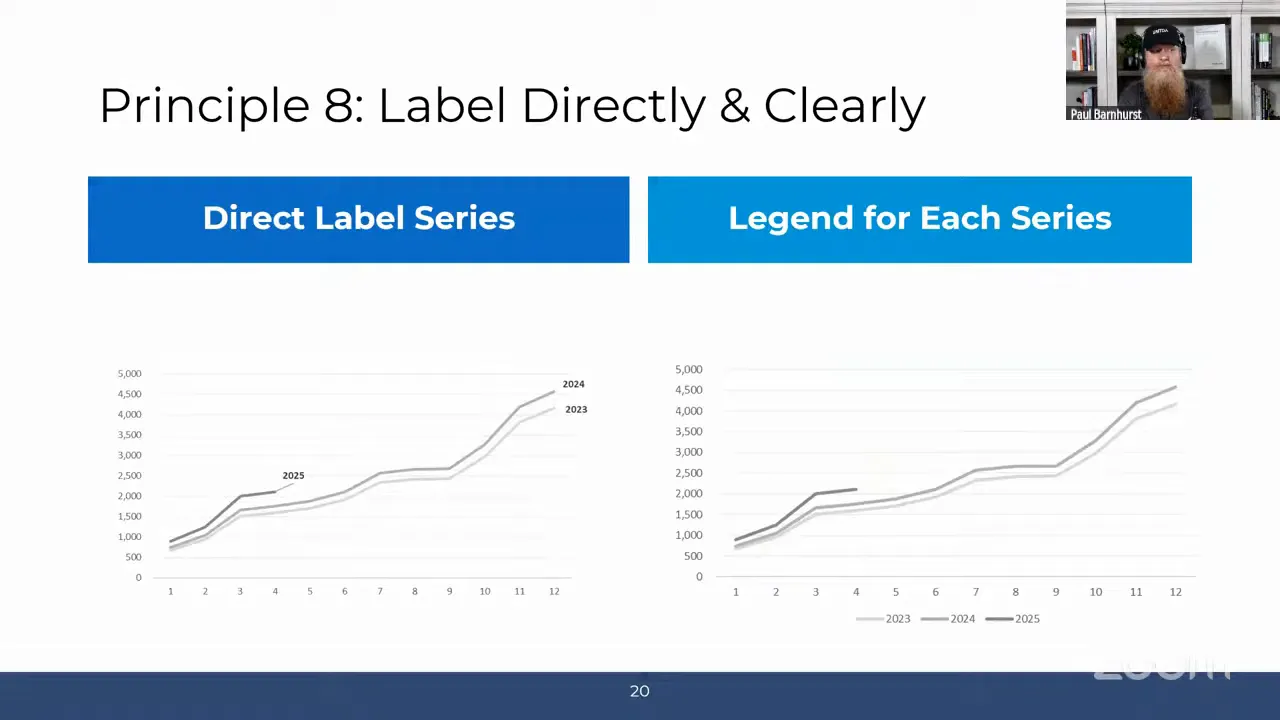
Direct labeling is one of the practical uses of NA() we will build shortly.
9. Choose the chart for the question
Start with the relationship you want to highlight, rather than a favorite chart type.
- Comparison: bar charts, column charts, and waterfall charts are useful options. Waterfalls are particularly familiar in financial planning and analysis.
- Correlation: scatter plots, heat maps, and bubble charts can reveal relationships.
- Parts of a whole: treemaps can provide a helpful overview of categories and subcategories. Pie charts have their place, but I use them sparingly.
- Change over time: line charts, stacked area charts, and candlestick charts suit different questions.
- Distribution: histograms and box plots help show how values are spread.
The same data can support several different charts. The right choice depends on what you want to make clear.
10. Provide context
An upward trend is not automatically good news. If the metric is the number of speeding tickets I receive each month, we have a problem.
Explain what the metric represents and give people something meaningful to compare it with:
- A historical period.
- A target, budget, or forecast.
- A benchmark.
- A threshold.
Without context, people fill in the gaps themselves, and they may reach very different conclusions.
Use Excel Tables as the Foundation
Before introducing NA(), there is one simple improvement I recommend for charts that need regular updates: build them from an Excel Table.
A chart linked to an ordinary fixed range may not pick up newly added months. You may also need to extend formulas, repair references, and copy formatting.
A Table makes that process much easier. As you add rows, its formatting and calculated columns extend, and a chart based on the Table can pick up the additional data.
For a one-time chart, a normal range may be perfectly adequate. For a recurring monthly report, a Table is usually worth the small amount of setup.
Tables and dynamic arrays are not competing approaches, either. A Table can hold the source data while a dynamic array filters or summarizes it for the chart.
What the NA() Function Does in Excel Charts
The syntax could hardly be simpler:
=NA()
There are no arguments. The function returns the #N/A error.
For the chart techniques here, that error has a useful purpose: it prevents an unwanted numeric point from being plotted. You retain the structure of a helper series without filling every position with a visible value.
This matters because a formula returning an empty string is not the same as a genuinely empty cell. Depending on the chart and its settings, apparently blank results can appear as zeros or otherwise produce an unwanted result.
Use NA() when a point does not belong in a particular chart series, rather than substituting zero. Zero is a real value, and plotting it can tell the wrong story.
A simple maximum-only helper series
Suppose your values occupy B2:B13. In a helper column, use:
=IF(B2=MAX($B$2:$B$13),B2,NA())
Copy it down. The formula returns the value when it equals the maximum and #N/A otherwise.
Now you have two series available:
- The original series containing every value.
- A helper series containing only the maximum value.
Format the helper series differently and you can highlight the maximum without manually selecting and recoloring a point each time the data changes. The same principle supports every example that follows.
Create Direct Labels That Follow the End of a Line
For a chart comparing 2023, 2024, and 2025, I would rather place each year beside its line than make people decode a legend.
The trick is to create a second, mostly invisible series for each year. Each helper series contains just the final relevant value, with NA() everywhere else.
Set up the endpoint helper series
- Keep the original data series for each year.
- Create a corresponding helper column for each series.
- Use lookup logic to identify the last populated position in the original series.
- Return the original value at that position and
NA()at all other positions. - Include both the original series and the helper series in the line chart.
The lookup needs to identify the last position, not the largest value. Those are different questions.
Label only the helper series
- Remove the legend if it is no longer needed.
- Select an endpoint helper series. If it is difficult to click, use the series selector on the chart’s Format tab.
- Add data labels to that helper series.
- Open Format Data Labels.
- Select Series Name and clear Value.
- Repeat for the remaining endpoint helper series.
- Position the labels neatly beside the line ends and remove unnecessary leader lines.
Make sure the helper series names contain the text you want displayed, such as the year.
Adding labels to the original series would label every point. Adding them to the helper series labels only the endpoint. As new months are included in the formula and chart source, the helper point moves and the label follows.
Show Actuals and Forecast as One Connected Line
This is one of my favorite uses of NA(). You can make a line look continuous while giving actuals and forecast different formatting.
Underneath, it is two separate series.
- Actuals: return the actual value for an actual period and
NA()otherwise. - Forecast: return forecast values for forecast periods, plus the final actual value at the transition.
The basic actuals formula follows this pattern:
=IF(ScenarioCell="Actuals",ValueCell,NA())
Replace the descriptive references with the relevant cells in your worksheet.
The forecast calculation needs one extra piece of logic: include the last actual point in the forecast series as well.
If actuals end in one month and forecast begins in the next, the two series do not share a point. That leaves a break. Including the final actual point in both series gives the forecast line somewhere to begin.
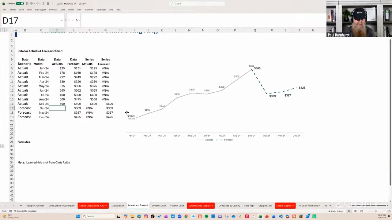
Once the series meet, format them independently. You can change the color, line weight, or dash style of the forecast without affecting the actuals.
As each new period becomes actual, the formulas move the transition. The example is financial, but the technique works anywhere you need two differently styled sections of a continuous trend.
Control Chart Series with Checkboxes and NA()
Checkboxes give people a straightforward way to choose what appears in a chart.
For example, you might always display sales while allowing people to add or remove cost of goods sold, gross profit, or customer counts. The same idea could let someone choose which stores to compare.
The checkbox returns TRUE or FALSE. A helper series translates that choice into chart data:
=IF(CheckboxCell,SourceValue,NA())
- When the checkbox is selected, return the source value.
- When it is cleared, return
NA().
Apply the logic to all points in each optional series, then build the chart from those helper ranges. Keep any series that should always appear linked directly to its values.
In Excel versions with in-cell checkboxes, select the control cells and use Insert > Checkbox. That is much simpler than setting up the older form controls for this kind of example.
Could you use a PivotChart instead? Absolutely. This is an alternative, not a declaration that every interactive chart should use formulas. Choose the approach that fits the data and the people maintaining the workbook.
Build Dynamic Charts with Spilled Arrays
NA() controls whether a point appears within a series. Dynamic arrays give you another useful option: change the dataset feeding the chart.
Create a top-N chart with SEQUENCE, FILTER, and LARGE
Suppose you have country data and want a dropdown that switches between the top five, top ten, or another number of countries.
- Create the list of available choices with
=SEQUENCE(25). - Use that spilled list as the source for a data validation dropdown.
- Add the spill operator,
#, to the source reference. For example, if the sequence starts inH2, use=$H$2#. - Use
LARGEto calculate the value at the selected rank. - Use
FILTERto return the rows meeting or exceeding that value. - Build the chart from the resulting dynamic output.
For a two-column dataset in A2:B101, with the numeric values in column B and the selected count in E2, the filtering logic is:
=FILTER(A2:B101,B2:B101>=LARGE(B2:B101,E2))
LARGE establishes the cutoff. FILTER returns the qualifying rows. Because the comparison includes equality, tied values at the cutoff can produce more than the selected number of rows.
The filter retains the source order, so use data ordered appropriately for a ranked display. In a horizontal bar chart, you can also select Categories in reverse order so the largest item appears at the top.
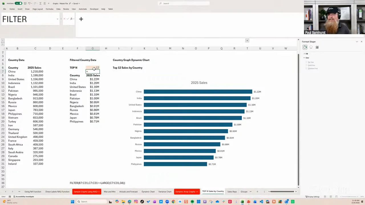
Then clean up the chart:
- Remove unnecessary gridlines and borders.
- Add value labels outside the bars.
- Use a meaningful title.
- Adjust the gap width to avoid overly thin bars.
I often use a gap width somewhere around 50% to 70%, with 60% as a reasonable starting point. That is a preference, not a law of chart design.
Filter selected rows with checkboxes
You can also combine checkboxes with FILTER to include only selected sales representatives.
The formula follows this pattern:
=FILTER(DataRange,CheckboxRange=TRUE)
The checkbox range supplies the inclusion test. Checked rows appear in the spilled output, and the chart adjusts with it.
You can omit =TRUE because the checkbox values are already Boolean. I often leave it in when teaching because it makes the logic more obvious.
Notice the distinction between the two checkbox methods:
- IF with NA(): keep the helper series structure and suppress unwanted points.
- FILTER: return only the selected rows to the chart’s source area.
Summarize a Table with GROUPBY
A third option combines an expanding source Table with a dynamic summary.
Use GROUPBY to group the records by product category and sum quantity or revenue. Configure the result to show headers, omit totals, and sort by the summarized measure.
One detail is easy to miss: the sort number identifies the output column as well as the direction.
If category is the first output column and summed quantity is the second:
-2sorts by quantity in descending order.2sorts by quantity in ascending order.-1sorts by the first column, not by quantity.
A result can accidentally look correctly ranked with the wrong sort argument. Change a value to test it rather than assuming the initial appearance proves the formula is right.
With the source in a Table, adding another month’s records expands the data, recalculates the summary, and updates the chart based on that summary.
Create an Interactive Bubble Chart
A bubble chart is useful when you genuinely need to communicate three measures together. In this example:
- Horizontal position: revenue.
- Vertical position: an EBITDA percentage measure.
- Bubble size: headcount.
That is three data dimensions, rather than a reason to add decorative 3D effects. In general, I would consider using two simpler charts before asking somebody to interpret three measures at once. A well-labeled bubble chart can be a useful exception.
Prepare the selectable data
Create a checkbox for each country, then build helper columns for the three numeric measures. Each helper formula returns the original measure when selected and NA() otherwise.
Lock the checkbox reference appropriately if you intend to copy the formula across all three measure columns.
During setup, select every country. It is easier to assess axis limits, spacing, and labels with the full dataset present. You can reduce the selection afterward.
Insert and format the chart
- Select the country labels and the three numeric helper columns, leaving out the checkbox selector and manager information.
- Insert a bubble chart from the scatter and bubble chart options.
- Check that Excel has assigned the correct ranges to horizontal values, vertical values, and bubble size. In this example, excluding the header row helped Excel interpret the selection correctly.
- Set sensible axis bounds. For the positive revenue data here, a horizontal minimum of zero removes unnecessary negative space.
- Adjust the percentage axis to suit the data.
- Add clear axis titles.
- Remove unnecessary gridlines and borders.
Add country names and headcount labels
In Format Data Labels, select Bubble Size to display headcount. Then use Value From Cells and select the country-name range.
Position the labels above the bubbles. If you want the country and headcount on separate lines, change the label Separator to New Line.
Under the series fill options, Vary colors by point gives the bubbles different colors.
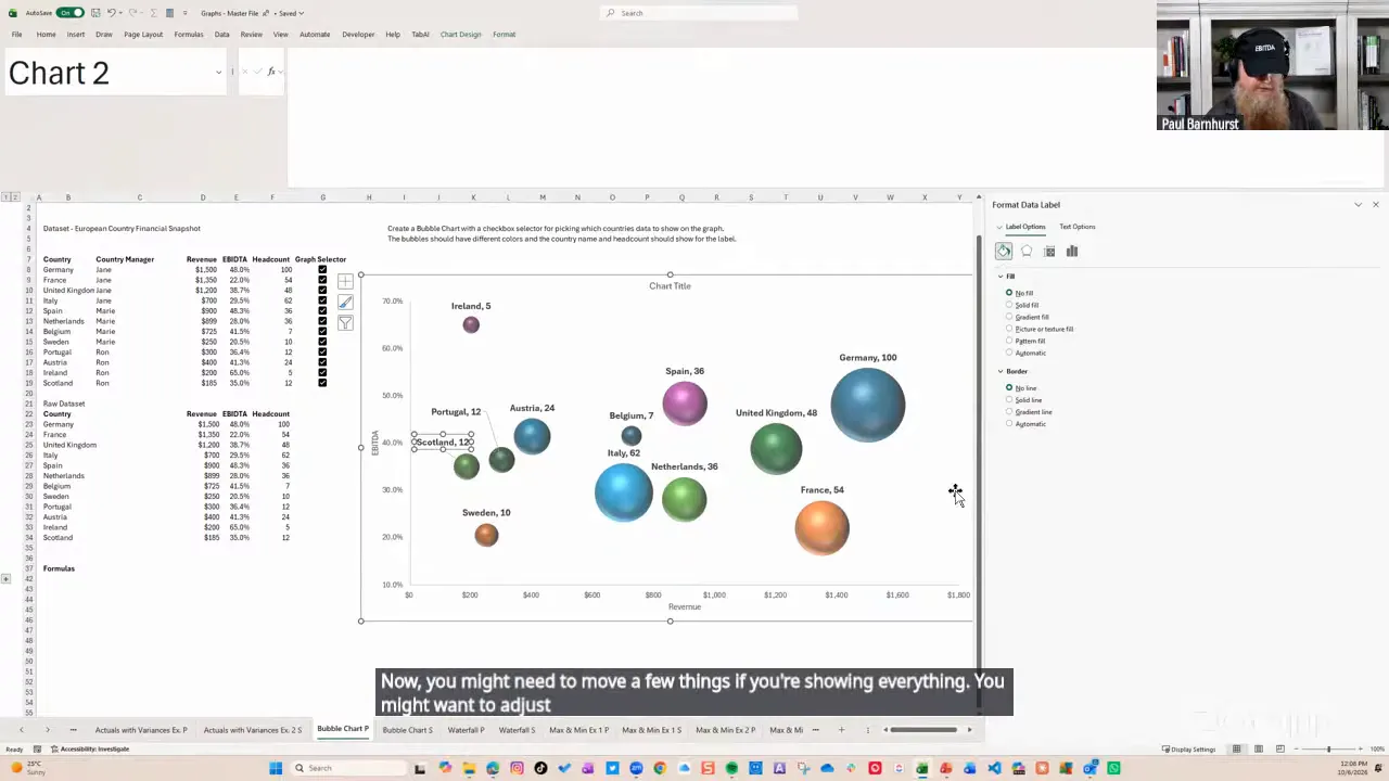
Now clear the countries you do not need. You can focus the discussion on a smaller set, such as the countries managed by one person, rather than presenting every bubble at once.
Varying colors by point does not automatically assign a consistent color to each manager. For a small, stable set, manually formatting individual bubbles may be sufficient. Do not confuse that point-color setting with a category-based coloring rule.
Show Actual Values with a Separate Variance Display
Putting two years of columns side by side often forces people to calculate the change mentally. I prefer an alternative that shows current values above and percentage movement below.
It is actually two charts aligned together:
- A column chart for current-year actual values.
- A scatter chart using error bars to draw positive and negative variance bars.
The separate positive and negative helper series give you control over colors, labels, and positioning.
Calculate positive and negative growth separately
In the example, current-year values are in column C and prior-year values are in column D. The positive helper formula is:
=IF(C8/D8-1>0,C8/D8-1,NA())
The negative helper formula is:
=IF(C8/D8-1<0,C8/D8-1,NA())
Each nonzero change appears in one of the two series. An exact zero is omitted by both tests.
Build the actuals chart
- Select the category labels and current-year values only.
- Insert a clustered column chart.
- Use a neutral fill, such as dark gray, so the variance colors can carry the emphasis.
- Add data labels above the columns.
- Remove unnecessary gridlines and value-axis labels.
- Make the chart wide enough for horizontal category labels.
- Set the chart area to No Fill and No Outline.
I avoid diagonal category labels where possible. They make people work harder than necessary.
Build the variance chart with error bars
Use matching horizontal category positions for the positive and negative variance series in an XY scatter chart. The two series must share those positions so they line up with the actuals columns.
For each variance series:
- Add error bars.
- Remove the horizontal error bars.
- Format the vertical error bars with Direction: Minus, End Style: No Cap, and Percentage: 100%.
- Hide the scatter series line and markers, leaving the vertical error bars visible.
- Increase the error-bar line width to make them look like narrow bars. A width of about 10 points was used here.
- Add data labels, placing positive labels above and negative labels below.
- Format the two series and their labels with distinct, purposeful colors.
The 100% error bars extend each variance point back to zero. Because positive and negative changes are separate series, you can format them independently.
Keep the zero baseline where it helps interpretation, but hide unnecessary axis labels. Make the chart background transparent, align it beneath the actuals chart, and group the two chart objects so they move together.
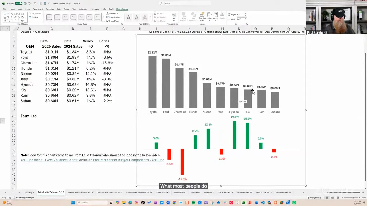
The initial alignment takes some manual adjustment. Once it is built, however, you can reuse the layout rather than rebuilding the scatter chart every month.
This method gives me the formatting control I want. It is not the only way to create a variance chart.
Automatically Highlight Maximum and Minimum Values
This final example brings together Tables, NA(), and overlapping chart series. It is practical, relatively simple, and useful in recurring reports.
Create the helper columns
Start with a Table containing month and gross sales. Add maximum and minimum helper columns.
Inside the Table, the maximum formula follows this structure:
=IF([@[Gross Sales]]=MAX([Gross Sales]),[@[Gross Sales]],NA())
The minimum formula is:
=IF([@[Gross Sales]]=MIN([Gross Sales]),[@[Gross Sales]],NA())
Use your actual column heading in place of Gross Sales.
You now have three series:
- Gross sales: every value.
- Maximum: the highest value, with
#N/Aelsewhere. - Minimum: the lowest value, with
#N/Aelsewhere.
Overlap the three series
- Select the month column and all three numeric series.
- Insert a Clustered Column chart.
- Check Change Chart Type and make sure all three series are clustered columns.
- Open Format Data Series with Ctrl+1.
- Set Series Overlap to 100%.
- Adjust the gap width, using about 70% as a starting point.
- Format the full sales series in gray.
- Give the maximum and minimum helper series distinct highlight colors.
The helper columns sit directly over the base columns. Where a helper contains #N/A, there is no highlight column. Where it contains the maximum or minimum, its colored column covers the gray one.
Add labels once
Add data labels to the original sales series only. The helper series repeat those same values, so labeling all three would create unnecessary duplicates.
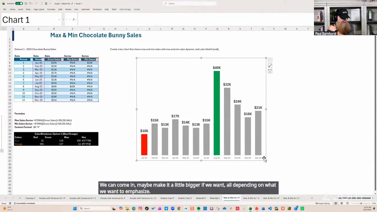
Change a sales value and the highlights move automatically. Add another month to the Table and the formulas and chart expand with it.
Ties work, too. If two months share the maximum, both satisfy the formula and both receive the maximum highlight.
The chart is not applying conditional formatting to individual points. It is switching which points exist in separately formatted series. That distinction is the key to understanding how the technique works.
Keep Color Automation Proportionate
There is a difference between automatically highlighting a value and automatically reading a fill color from a worksheet cell.
The maximum and minimum chart automates the highlight through formulas and series membership. It does not need to change a point’s fill dynamically.
For fixed colors, you can enter a hex value or RGB values through More Fill Colors. For a consistent workbook palette, custom theme colors under Page Layout can help establish a repeatable accent order.
If you need chart fills to respond directly to color codes stored in cells, that is a different automation task and may involve VBA. For a small number of stable elements, I often format them manually. A minute of setup that stays correct can be more sensible than building an elaborate solution.
Make the Message Easier to See
The common thread is simple: separate the data you have from the data each chart series needs to display.
NA() supplies the missing points. Tables make recurring source data easier to maintain. Dynamic arrays reshape the chart input. Checkboxes let people focus on the comparison they need.
But none of those tools replaces the design question: What should this chart help somebody understand or decide?
For more on that side of the work, I recommend Storytelling with Data, Stephen Few’s Show Me the Numbers, Nick Desbarats’ Practical Charts, and Brent Dykes’ Effective Data Storytelling.
There are clear bad practices, but there is also room for judgment. Use the techniques that make your message clearer, remove what does not help, and do not make somebody decode a wall of numbers when a thoughtful visual can make the issue obvious.


