I find myself using the HSTACK function in Excel every day, which is far more than I expected when it first appeared. It sounds like a fairly simple function: give it some arrays, and it puts them side by side.
But that simple job becomes incredibly useful when you start combining it with FILTER, LET and GROUPBY. HSTACK can bring quarterly sales together, make column selections easier to read, combine separate calculations into one report, and even supply multiple functions to a grouped summary.
You can follow along with the HSTACK practice workbook.
What You'll Learn
- HSTACK combines matching quarterly sales ranges across consecutive worksheets into one annual report.
- Explicit table-column references make HSTACK a readable alternative to CHOOSECOLS inside FILTER.
- LET and HSTACK combine separate calculations into a single report output.
- HSTACK supplies multiple aggregation functions to GROUPBY, while DROP removes the extra header row.
1. Combine Quarterly Sales Across Worksheets
HSTACK is Excel’s horizontal stacking function. It combines columns or arrays side by side. There is also a VSTACK function for stacking arrays vertically.
The basic structure is straightforward:
=HSTACK(array1, array2, ...)The interesting part is how we supply those arrays.
For this first example, there are four worksheets named Q1, Q2, Q3 and Q4. Each contains employee and department information, with that quarter’s sales in column D. Crucially, the sales occupy the same cell range on every sheet, and the quarterly sheets are consecutive in the workbook.
That layout gives us a very neat way to combine the sales:
- Select the output cell beside the employee and department details on the combined report.
- Type
=HSTACK(. - Click the Q1 worksheet and select the sales range in column D.
- Hold Shift and click the Q4 worksheet tab.
- Close the bracket and press Enter.
Shift-clicking the final quarter creates a reference spanning Q1 through Q4. HSTACK then places each quarter’s sales column beside the previous one, giving us the entire year in a single output.
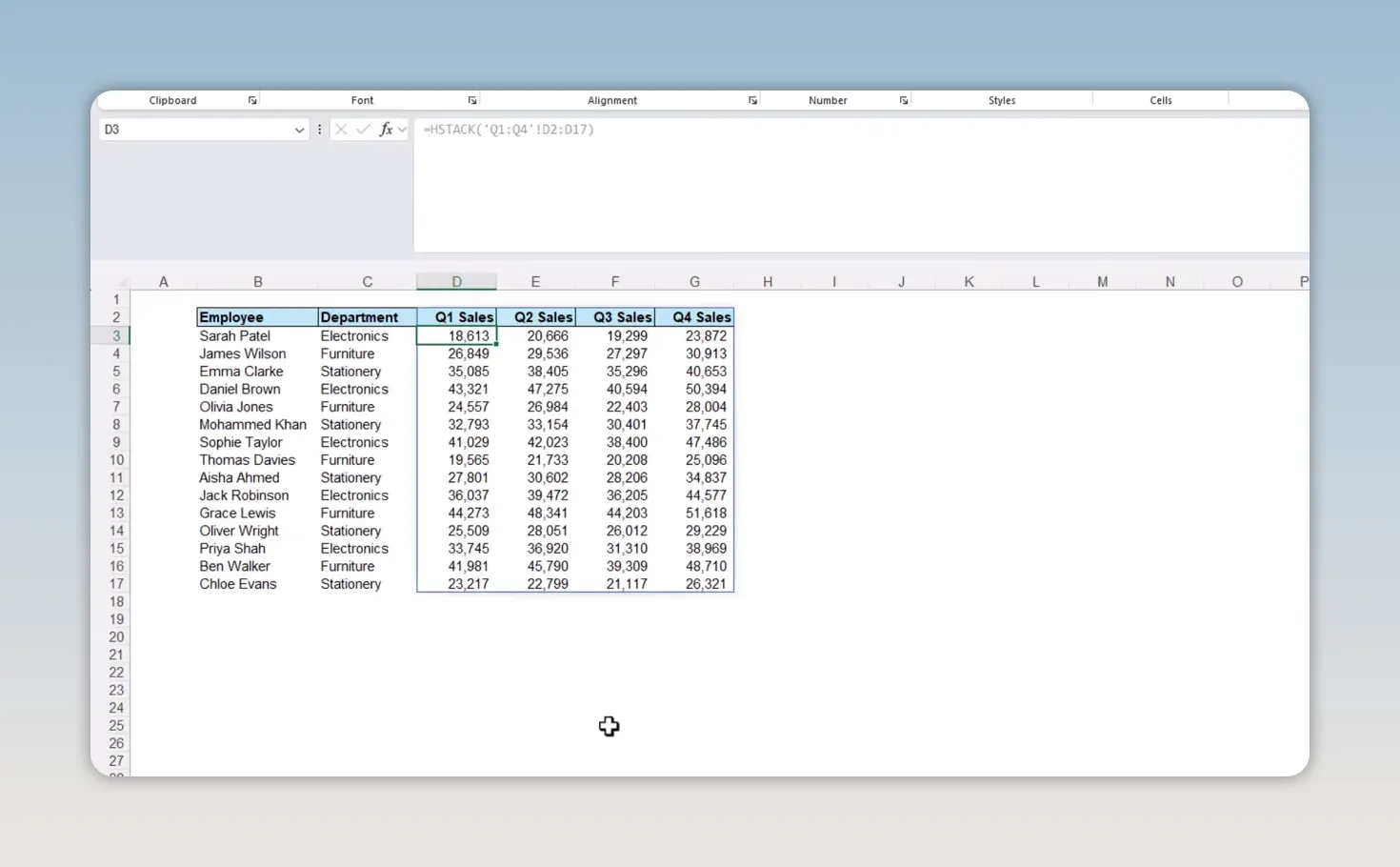
I’m a huge fan of Excel tables. They are the foundation of so much good Excel work. However, this is a useful exception where ordinary ranges let us take advantage of an identical layout across consecutive worksheets.
The layout matters here. HSTACK places the ranges beside each other, so the employee rows need to correspond across the quarterly sheets.
2. Use HSTACK Instead of CHOOSECOLS for Readable Column Selections
The next example uses a six-column Excel table named tblStock, containing product details and stock levels.
The report needs to return only products with stock below the threshold in cell D2, which is set to 50. It also needs just three columns:
- Product Name
- Category
- Stock Level
A classic solution is to use CHOOSECOLS inside FILTER. CHOOSECOLS selects the second, third and fifth columns, and FILTER keeps the products below the threshold:
=FILTER(
    CHOOSECOLS(tblStock,2,3,5),
    tblStock[Stock Level]<D2
)
That works perfectly well. CHOOSECOLS does exactly what its name suggests, and column numbers can be useful in more dynamic solutions.
However, 2, 3 and 5 do not tell me much about the columns being returned. HSTACK gives us a nice alternative:
=FILTER(
    HSTACK(
        tblStock[Product Name],
        tblStock[Category],
        tblStock[Stock Level]
    ),
    tblStock[Stock Level]<D2
)
The result is the same, but the formula is now explicit. I can immediately see that it returns the product name, category and stock level, in that order.
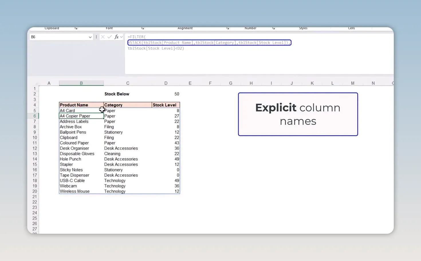
Rather than counting column positions, I can select the table columns directly while building the formula. I also do not need to use the report’s headings to look up matching source-column names.
I often find that AI tools such as Copilot and ChatGPT suggest HSTACK when returning particular columns from a dataset. This is a good example of why that approach can be useful: the formula clearly communicates what it is doing.
CHOOSECOLS is not wrong here. HSTACK is simply another option, and one I particularly like when readability is the priority.
3. Build a Single-Formula Report with LET and HSTACK
HSTACK becomes especially useful when the columns we want to display are not simply existing columns from one dataset.
For this report, I want four pieces of information together:
- The month and year.
- Revenue for 2026.
- Revenue for 2025.
- The variance between those revenue values.
The revenue calculations come from completely different tables. I have used LET to perform the separate calculations and assign a name to each result:
monthYearsrevenue2026revenue2025yearVar
If LET is new to you, its purpose here is to give meaningful names to intermediate calculations within a formula. Microsoft’s LET function reference explains that structure in more detail.
Initially, the final argument of the LET formula returns only monthYears. The other calculations have been defined, but they are not yet included in the report output.
We can replace that final argument with this HSTACK expression:
HSTACK(monthYears,revenue2026,revenue2025,yearVar)This is the final expression inside the existing LET formula, not a separate formula relying on worksheet names. HSTACK takes the four calculated arrays and combines them into one output.
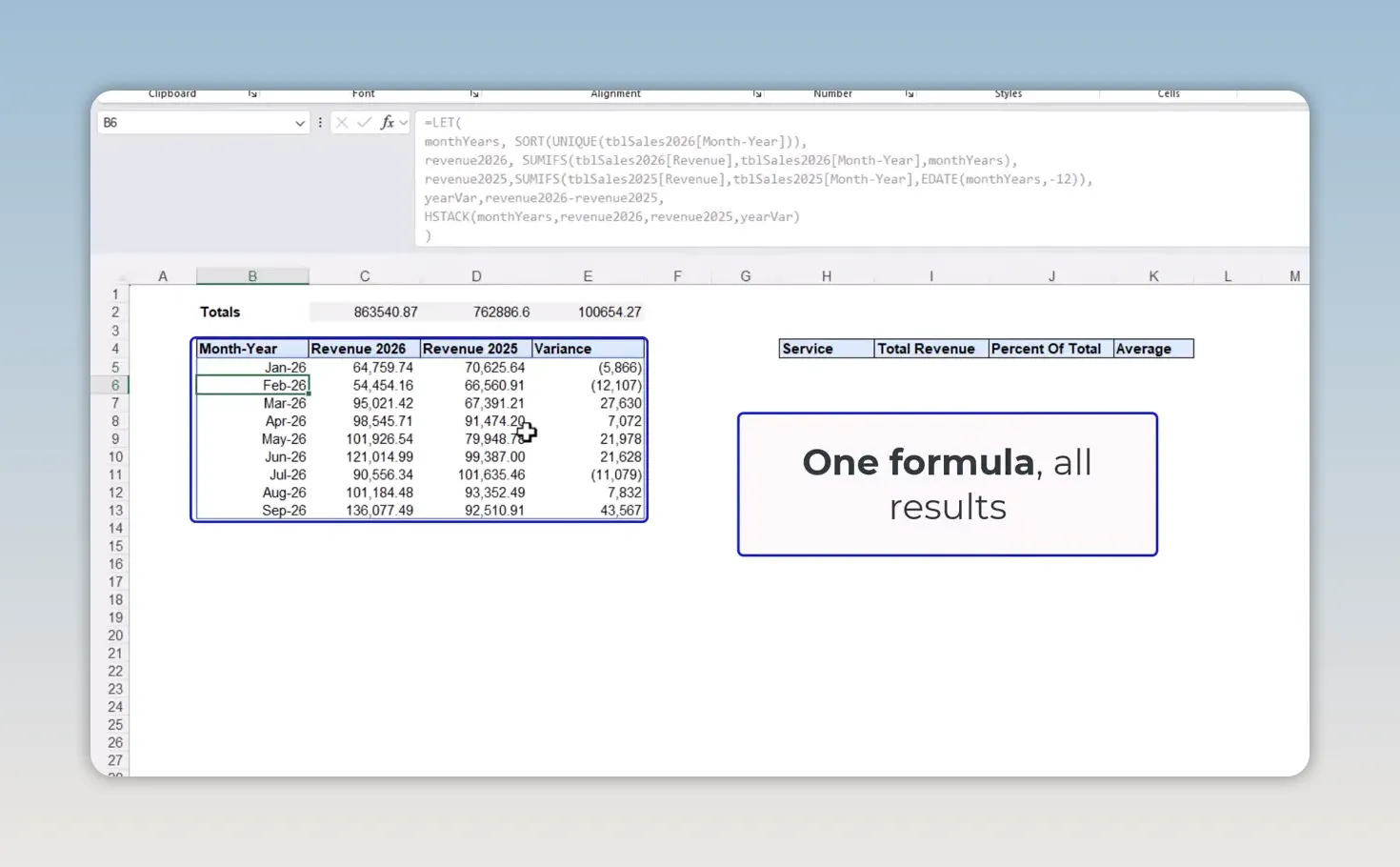
This is why I find HSTACK so useful for formula-based reports. LET handles the calculations and gives them names. HSTACK arranges their results into the columns I want.
If I make an additional calculation, I can add its named result to HSTACK rather than create a separate output formula beside the report.
For more on building formulas like this, my Next-Gen Excel Formulas course covers dynamic arrays, modern lookups, LET and LAMBDA.
|

4. Supply Multiple Functions to GROUPBY with HSTACK
The final example is a particularly interesting use of HSTACK. Rather than combining data columns or calculated results directly, we use it to supply multiple aggregation functions to GROUPBY.
Using the tblSales2026 table from the revenue report, I want to group the records by service and calculate three measures from the Revenue column:
- SUM: total revenue for each service.
- PERCENTOF: each service’s percentage of the total revenue.
- AVERAGE: average revenue within each service group.
GROUPBY takes the Service column as its grouping field and Revenue as the values to calculate. For its function argument, we can supply HSTACK(SUM,PERCENTOF,AVERAGE):
=GROUPBY(
    tblSales2026[Service],
    tblSales2026[Revenue],
    HSTACK(SUM,PERCENTOF,AVERAGE)
)
Notice that SUM, PERCENTOF and AVERAGE are supplied as function names, without their own argument lists. GROUPBY applies them to the grouped revenue values.
There is a small quirk worth knowing about: Excel may not offer HSTACK in its suggestions at this point. That can give the impression that this combination is not available. It absolutely works, so keep typing the expression manually.
The function names do not need to be capitalised. I enter them that way out of habit.
Remove the Extra Header Row with DROP
When GROUPBY returns these multiple calculations, it also produces a row of function headings. That is useful in some reports, but I already have my own headings above the output.
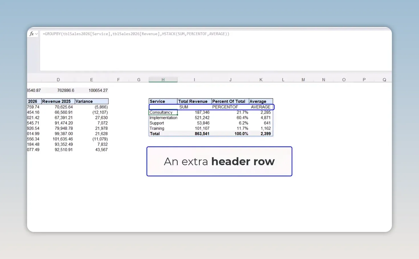
Wrapping the calculation in DROP removes that first row:
=DROP(
    GROUPBY(
        tblSales2026[Service],
        tblSales2026[Revenue],
        HSTACK(SUM,PERCENTOF,AVERAGE)
    ),
    1
)
The 1 tells DROP to remove one row from the top of the result, leaving the grouped calculations beneath my existing report headings.
For more detail on these supporting functions, see my tutorials on TAKE and DROP and the PERCENTOF function.
A Simple Function That Fits into Bigger Formulas
HSTACK is easy to understand, but its usefulness goes well beyond joining a couple of columns. It can combine matching ranges across worksheets, make a FILTER formula easier to read, assemble a report from named calculations, and supply several functions to GROUPBY.
That is why I keep using it. The individual calculations may be quite different, but I so often need their results side by side. HSTACK gives me a straightforward way to bring them together.


