GROUPBY and PIVOTBY are brilliant for building formula-based summaries in Excel. But there is one PivotTable feature I am frequently asked about: how do you drill down to the transactions behind a result?
With a PivotTable, you can double-click a value to display its underlying records on a new worksheet. Excel calls this Show Details, although drill down is the name most of us use.
We can create a similar experience for a formula-based report. I will show you two approaches: one using a tiny piece of VBA, and another using checkboxes, data validation, FILTER and XLOOKUP, with no VBA at all.
Both approaches use hyperlinks to navigate to a details sheet. A single click is a nice alternative to the double-click action of a PivotTable, particularly on modern devices.
You can use the practice workbook to work through the examples.
Table of Contents
- Start with a GROUPBY Summary
- Method 1: Add Drill Down with a Small VBA Procedure
- Method 2: Create Drill Down Without VBA
- Which Drill-Down Method Should You Use?
Start with a GROUPBY Summary
Imagine a sales report listing products and their total sales. In a PivotTable, double-clicking the total for a product such as XL Iced Nitro produces the transaction rows contributing to that sum.
To create the summary with a formula instead, use GROUPBY. The source data in this example is an Excel table named tblSales, containing columns named Product Name and Total Sales.
=GROUPBY(tblSales[Product Name],tblSales[Total Sales],SUM)The three arguments tell Excel to:
- Group the records by product name.
- Use the total sales column as the values.
- Add those values together using SUM.
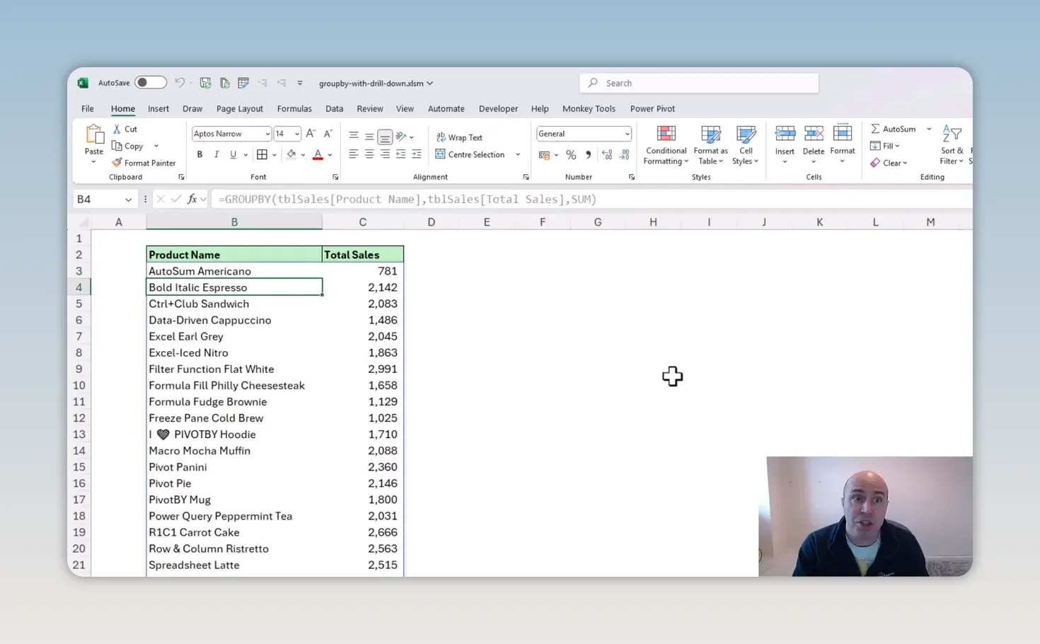
That gives us a formula-based interpretation of the PivotTable. What we still need is a way to select a product and display its original sales records.
The same selection-and-filtering idea can support a PIVOTBY report. The worked example here uses a product-only GROUPBY summary, so the details criteria are based on one product name.
Method 1: Add Drill Down with a Small VBA Procedure
The VBA approach is the more straightforward of the two. A worksheet event captures the selected product name, places it in a cell on the details sheet, and lets FILTER do the rest.
There are some limitations to bear in mind. Some organisations restrict VBA for security reasons, and VBA does not run in Excel for the web. If either applies to your report, use the checkbox method later in this article.
1. Build the details sheet with FILTER
Create a worksheet for the transaction details. Use cell C2 to hold the product name you want to investigate.
Below it, add the source column headings and enter this formula in the first cell beneath those headings:
=FILTER(tblSales,tblSales[Product Name]=C2,"No product specified")This returns all columns from tblSales, but only for records where the product name matches C2. The final argument supplies a message if there are no matching rows.
Try entering a different product name in C2. The records change immediately. That is our details page working already. We simply need to connect it to the summary.
If FILTER is new to you, Microsoft’s FILTER function reference explains its array, include and empty-result arguments.
2. Add hyperlinks to the product names
Return to the worksheet containing GROUPBY and select the product-name cells in the results, excluding headings and any total row.
- Choose Insert > Link.
- Select Place in This Document.
- Choose the details worksheet as the destination.
- Confirm the link.
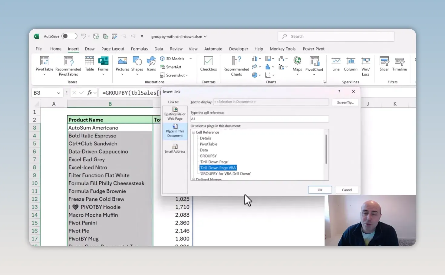
All of these links can lead to the same details worksheet. The hyperlink handles navigation; the VBA will identify which product was selected.
Excel may apply hyperlink formatting to the product names. If you prefer the original report appearance, select those cells and choose Home > Cell Styles > Normal. The links remain in place even though the text no longer has the usual hyperlink appearance.
3. Capture the selected product with VBA
Open Developer > Visual Basic and open the worksheet code module for the sheet containing the GROUPBY formula.
The event we need is Worksheet_SelectionChange. Its Target argument identifies the selected cell.
The essential instruction is just this:
drilldown.Range("C2").Value = Target.ValueHere, drilldown is the VBA code name assigned to the details worksheet, not simply the name displayed on its sheet tab. The instruction copies the selected cell’s value into C2 on that sheet.
For a practical implementation, limit the event to single-cell selections within the product-name range. For example, if your product names occupy B5:B29:
Private Sub Worksheet_SelectionChange(ByVal Target As Range)

    If Target.CountLarge > 1 Then Exit Sub
    If Intersect(Target, Me.Range("B5:B29")) Is Nothing Then Exit Sub

    drilldown.Range("C2").Value = Target.Value

End Sub
Change B5:B29 to match your report and use the correct code name for your details worksheet. The two checks keep unrelated selections and multi-cell selections out of the procedure.
Save the workbook in a macro-enabled format, such as .xlsm, and enable macros only when the workbook is trusted and your organisation permits them.
4. Test the drill-down action
Click a product hyperlink in the summary. The selection event transfers the product name into C2, the hyperlink takes you to the details sheet, and FILTER returns the matching transactions.
For example, selecting Filter Function Flat White displays its sales records. Returning to the summary and choosing R1C1 Carrot Cake changes the details to that product instead.
That is the Show Details effect with very little VBA. Unlike the standard PivotTable action, this setup reuses one details worksheet rather than creating a fresh worksheet each time.
Method 2: Create Drill Down Without VBA
Without VBA, the challenge is capturing the product selection. A hyperlink can take us to another worksheet, but it does not write the clicked cell’s value into our filter criterion.
My approach is to make the selection explicit with in-cell checkboxes. We can then use XLOOKUP to find the checked product and FILTER to return its transactions.
Start with the same GROUPBY summary and product hyperlinks, but point the links to a separate details worksheet for this version.
1. Insert checkboxes beside the products
Add a column to the left of the product names and give it a heading such as Show Details.
- Select the cells alongside the product names.
- Choose Insert > Checkbox.
- Click a checkbox to test it.
I love how easy these checkboxes are to use. More importantly, they are values we can use directly in formulas:
- An unchecked checkbox has the value
FALSE. - A checked checkbox has the value
TRUE.
Checking the box beside Formula Fill Philly Cheesesteak gives us a clear signal that this is the product whose details we want.
2. Prevent more than one checkbox being selected
At this stage, somebody could check several boxes. That could be useful for a different report, but our aim here is a single-product details page.
We can use data validation to allow no more than one checked box.
- Select the checkbox cells.
- Choose Data > Data Validation.
- Set Allow to Custom.
- Enter a formula that counts the checked boxes and requires the result to be no greater than one.
For a checkbox range of A5:A29, use:
=SUM($A$5:$A$29+0)<=1Adjust the range to match your worksheet. The absolute references ensure every checkbox is tested against the same complete range.
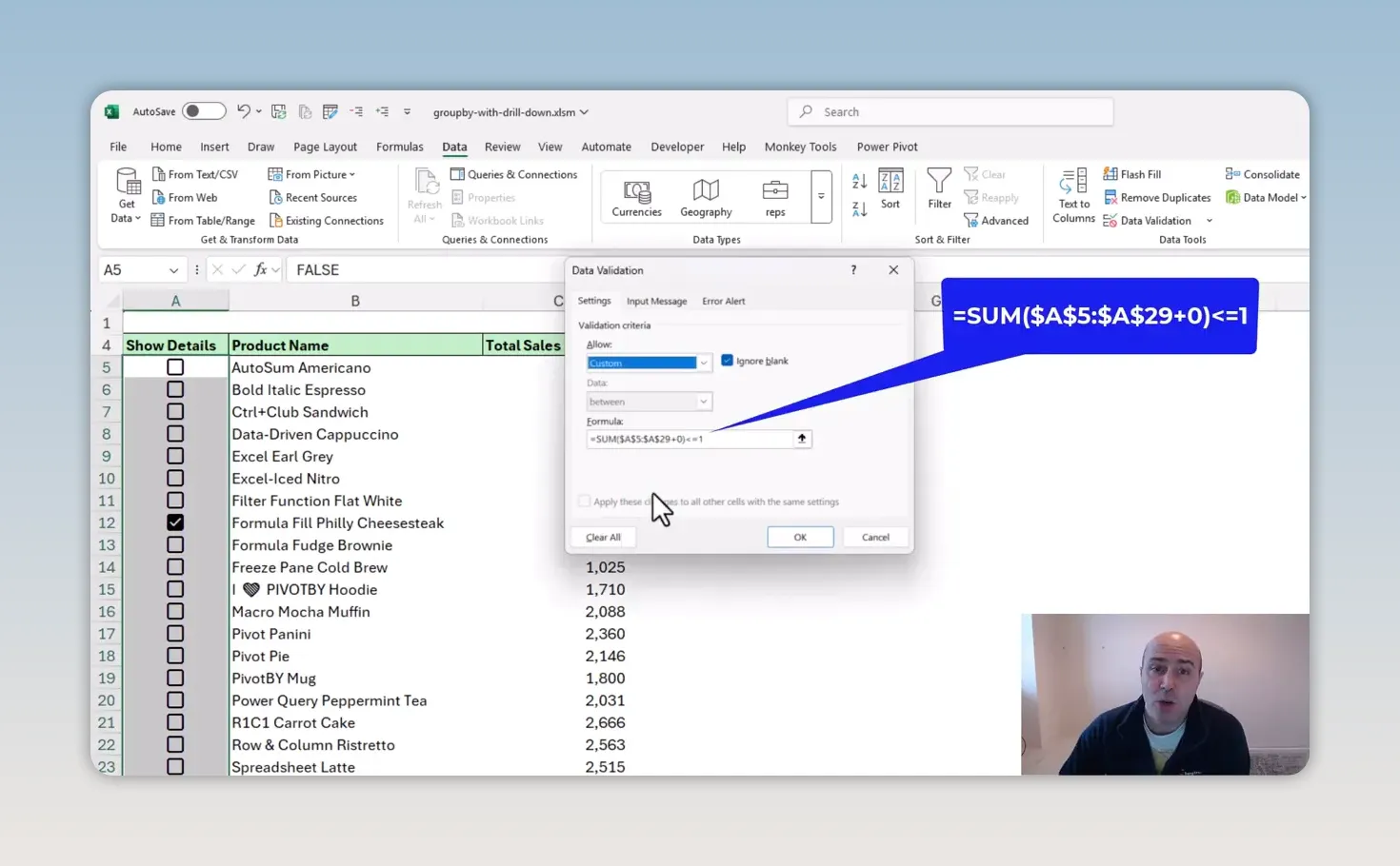
The +0 converts TRUE and FALSE into 1 and 0. SUM then counts the checked boxes, and <=1 allows either zero or one.
With the validation rule applied, checking a second box is blocked. To choose a different product, first clear the existing selection and then check the new one.
3. Name the checkbox and product ranges
Named ranges are not essential, but I like them because they make the upcoming formula much easier to read.
- Select the checkbox cells and name the range
rngCheckboxes. - Select the corresponding product-name cells and name the range
rngProductNames.
You can enter each name in the Name Box to the left of the formula bar, then press Enter.
Be careful not to activate a hyperlink while selecting the product names. Also make sure the two named ranges contain the same number of rows and line up correctly. Each checkbox must correspond to the product on the same row.
4. Use XLOOKUP to identify the checked product
On the details worksheet, XLOOKUP can search the checkbox range for TRUE and return the corresponding product name:
=XLOOKUP(TRUE,rngCheckboxes,rngProductNames)For example, if the Data Driven Cappuccino checkbox is selected, that is the product name returned by the lookup.
We can put this lookup directly inside FILTER instead of using a separate criterion cell.
5. Combine FILTER and XLOOKUP
Enter the following formula beneath the column headings on the details sheet:
=FILTER(tblSales,tblSales[Product Name]=XLOOKUP(TRUE,rngCheckboxes,rngProductNames,""),"No checked boxes")The formula works in three stages:
- XLOOKUP finds TRUE in
rngCheckboxesand returns the matching product fromrngProductNames. - The comparison identifies matching transactions in the source table’s product-name column.
- FILTER returns those transaction rows from
tblSales.
I have included an empty-string fallback, "", as XLOOKUP’s fourth argument. Without it, having no checked box produces a lookup error before FILTER can display its empty-result message. Assuming the source contains no blank product names, this fallback allows the formula to display No checked boxes when nothing is selected.
6. Test the checkbox-based drill down
Return to the summary and check the box beside Data Driven Cappuccino. Click its product hyperlink to open the details worksheet. The matching sales records are returned.
Now return to the summary, clear that checkbox, check the box beside PivotBy Mug, and follow its hyperlink.
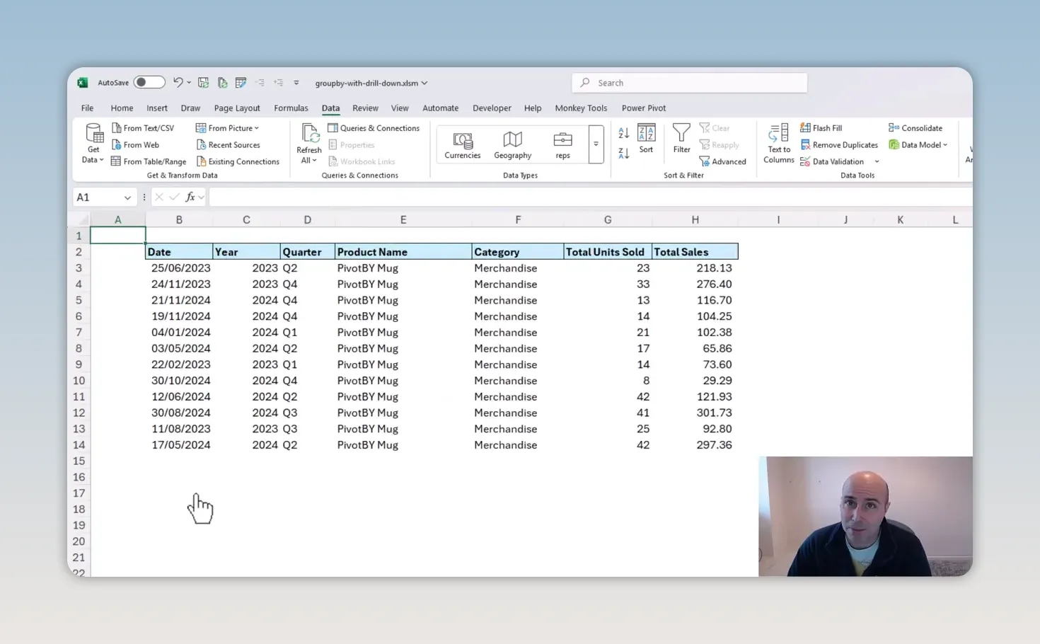
The details now show the PivotBy Mug transactions. No VBA required. Pretty awesome.
There is one important distinction: the checkbox determines the product, not the hyperlink you click. The links all navigate to the details sheet, while the formula reads the checked row.
Which Drill-Down Method Should You Use?
Both methods connect a formula-based summary to the records behind it, but they offer slightly different experiences.
- Use VBA for the simpler interaction. Selecting a product hyperlink supplies the product name and opens its details, provided macros are permitted.
- Use checkboxes when VBA is not an option. The selection is stored in worksheet cells and read using formulas, although changing products requires clearing the previous checkbox.
The checkbox approach also suggests an interesting extension: selecting several products and displaying their combined details. That would require different filtering logic, because the XLOOKUP formula here returns only the first checked product. Removing the validation rule alone would not create a multiple-product report.
For a single-product Show Details experience, however, we have everything we need: a GROUPBY summary, hyperlinks for navigation, FILTER for the transactions, and either a tiny VBA event or checkboxes with XLOOKUP to connect them. It is a lovely example of how Excel’s newer functions can work together to make reports more interactive.


