The IMPORTCSV function makes it incredibly easy to bring CSV data directly into an Excel worksheet. Give it a file path, press Enter, and the contents spill into the grid from a single formula. There is no need to open the CSV or copy and paste its contents.
Better still, because it is a formula, we can build the file path dynamically and combine the imported results with other Excel functions. A drop-down selection can determine which CSV to import, SUBSTITUTE can tidy up the filename, and DROP can remove a column we do not need.
Does this replace Power Query? Absolutely not. Power Query remains the go-to tool for data connections and transformations. IMPORTCSV offers a handy alternative for more lightweight, dynamic solutions.
Availability note: At the time of this demonstration, IMPORTCSV was available to Microsoft 365 Beta channel users only, with a wider release expected. Availability may depend on your Excel version and update channel.
What You'll Learn
- IMPORTCSV brings CSV data into the worksheet as a spilled array using one required file-path argument.
- Refresh All retrieves saved source-file changes; imported data does not update automatically.
- Combine IMPORTCSV with worksheet selections, SUBSTITUTE, and DROP to build dynamic import solutions.
- Specify the source locale to resolve regional date and number interpretation conflicts.
Table of Contents
- Import a CSV File into Excel
- Refresh IMPORTCSV When the Source Changes
- Import a CSV from SharePoint or OneDrive
- Choose Which CSV to Import with a Drop-Down
- Remove an Unwanted Column with DROP
- Fix Date Conflicts with the Source Locale
- When to Use IMPORTCSV Instead of Power Query
Import a CSV File into Excel
We will start with a CSV containing UK sales transactions. The only required argument for IMPORTCSV is the path to the file.
- Locate the CSV in File Explorer.
- Right-click the file and choose Copy as path.
- Return to Excel and select the cell where you want the imported data to begin.
- Type
=IMPORTCSV(and paste the copied path. - Close the bracket and press Enter.
Using an illustrative folder path, the formula looks like this. Replace the path with the location of your own CSV:
=IMPORTCSV("C:\Exports\sales_transactions_uk.csv")The path is text, so it needs double quotes around it. When using Copy as path, those quotes may already be included. If Excel displays the paste security prompt shown in the demonstration, choose Paste without active content.
That is all we need for a basic import. Excel returns the CSV contents as a spilled dynamic array, with one formula producing the entire result.
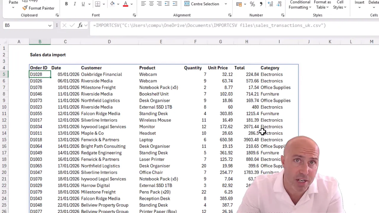
From there, you can reference the result from other formulas or use it with charts, just as you would with other spilled formula results.
What do the optional arguments do?
Although the path is the only mandatory argument, IMPORTCSV also provides options to refine the import:
- Rows to skip: Leave out rows at the beginning of the source.
- Rows to take: Limit the number of rows returned, such as taking only the first 10.
- Formatting options: Control how the imported data is handled.
- Locale: Specify the regional conventions used by the source data.
The locale option is particularly useful when a CSV uses different decimal separators or a different date structure from your regional settings. We will use that shortly to import US invoice dates into a UK workbook.
Refresh IMPORTCSV When the Source Changes
One important distinction: IMPORTCSV is refreshable, but source-file changes do not appear automatically.
For example, suppose the first sales transaction has a category of Electronics. Open the source CSV, change that category to Fruit, then save and close the file.
Back in the importing workbook, the result still shows Electronics. To retrieve the updated data:
- Select the Data tab.
- Choose Refresh All.
The imported result now shows Fruit.
So, although the data comes into the worksheet through a formula, you still need to refresh it to pick up changes saved in the source CSV.
Import a CSV from SharePoint or OneDrive
The path does not have to point to a local file. IMPORTCSV can also bring in data from a web URL, including a CSV stored on SharePoint or OneDrive.
For the OneDrive example, I use the online path available from the source file in Excel:
- Open the source CSV and go to File > Info.
- Use Copy path to copy its online location.
- In the destination workbook, enter IMPORTCSV and paste the online path inside double quotes.
- If the copied path ends with
?web=1, remove that suffix so the path ends with.csv. - Close the formula and press Enter.
The CSV data spills into the worksheet in the same way as the local-file example. The source location changes, but the basic approach remains the same: supply the CSV path as the first argument.
Choose Which CSV to Import with a Drop-Down
This is where using a formula gets particularly useful. Rather than hard-coding a filename, we can construct it from a cell value.
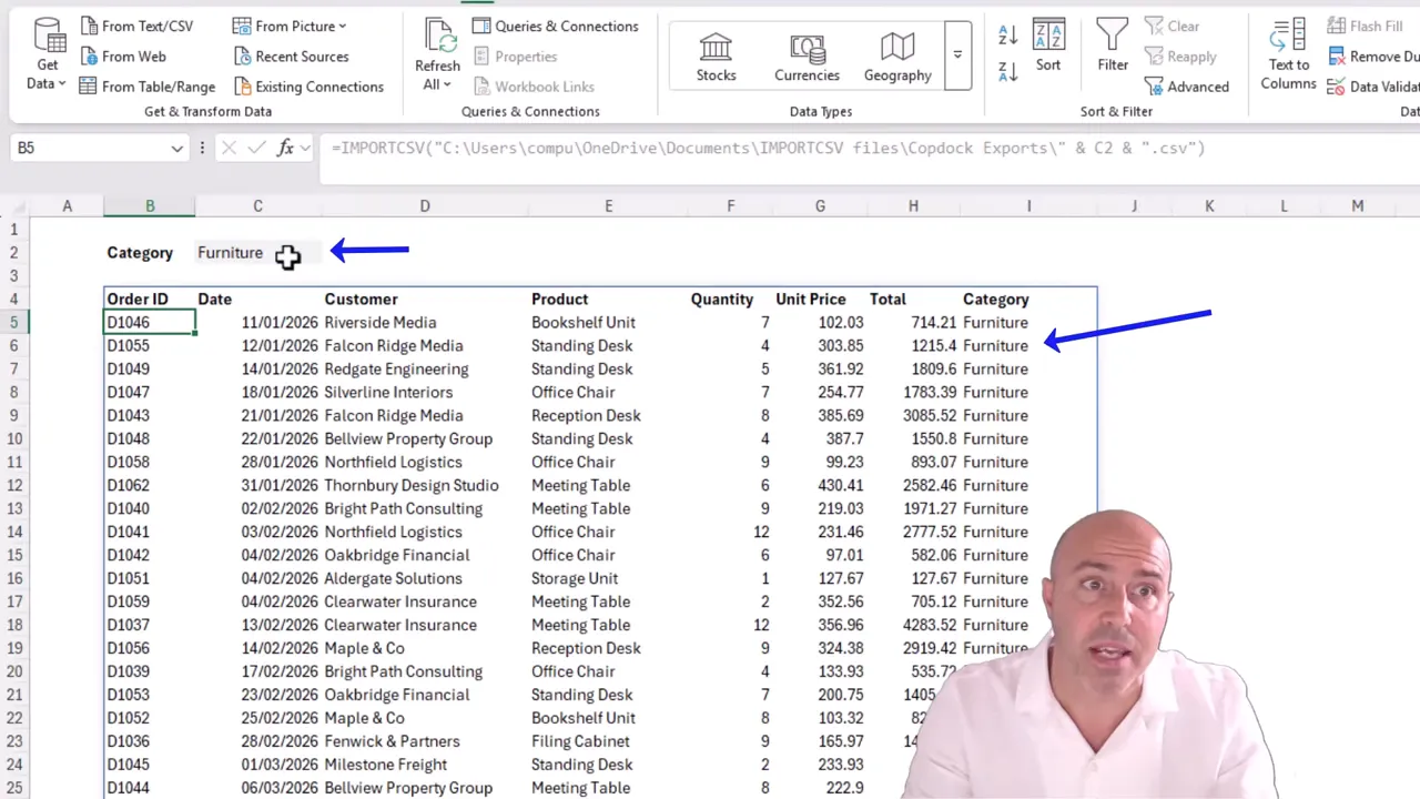
In this example, cell C2 contains a data validation drop-down with three categories:
- Furniture
- Electronics
- Office Supplies
A folder contains a separate CSV for each category. We want the selection in C2 to determine which file is imported.
There is no need to import all three files and then filter out the data we do not want. Instead, we build the appropriate source path directly.
Build the file path with ampersands
The path has three parts: the folder, the category selected in C2, and the .csv extension. Ampersands join those parts together.
Using an illustrative folder location, the formula is:
=IMPORTCSV("C:\Exports\Category Exports\" & C2 & ".csv")When C2 contains Furniture, the formula imports the Furniture CSV. Change C2 to Electronics, and the result switches to the Electronics data.
Fix a filename mismatch with SUBSTITUTE
Furniture and Electronics work nicely. But selecting Office Supplies produces a #VALUE! error in this example.
The reason is simple: the drop-down value contains a space, while the CSV filename uses an underscore: Office_Supplies.csv.
To make the selection match the filename, wrap the C2 reference in SUBSTITUTE:
=IMPORTCSV("C:\Exports\Category Exports\" & SUBSTITUTE(C2," ","_") & ".csv")The expression SUBSTITUTE(C2," ","_") takes the selected category, replaces spaces with underscores, and supplies the resulting text to the path.
Now Office Supplies imports the correct CSV as well.
This is the real benefit of working with a function. We can combine IMPORTCSV with SUBSTITUTE, LOWER, XLOOKUP, or whatever other functions the solution needs to construct the appropriate path.
Remove an Unwanted Column with DROP
The category files include a final Category column. That column is redundant here because the category is already selected in C2.
IMPORTCSV has arguments for skipping and taking rows, but it does not have a dedicated argument for removing that final column. We can handle it by wrapping the import in DROP:
=DROP(IMPORTCSV("C:\Exports\Category Exports\" & SUBSTITUTE(C2," ","_") & ".csv"),,-1)Here is how the outer function works:
- Array: The result returned by IMPORTCSV.
- Rows: Left blank because we do not want to remove rows.
- Columns: Set to
-1to remove one column from the end.
For the columns argument, a positive number removes columns from the beginning, while a negative number removes them from the end.
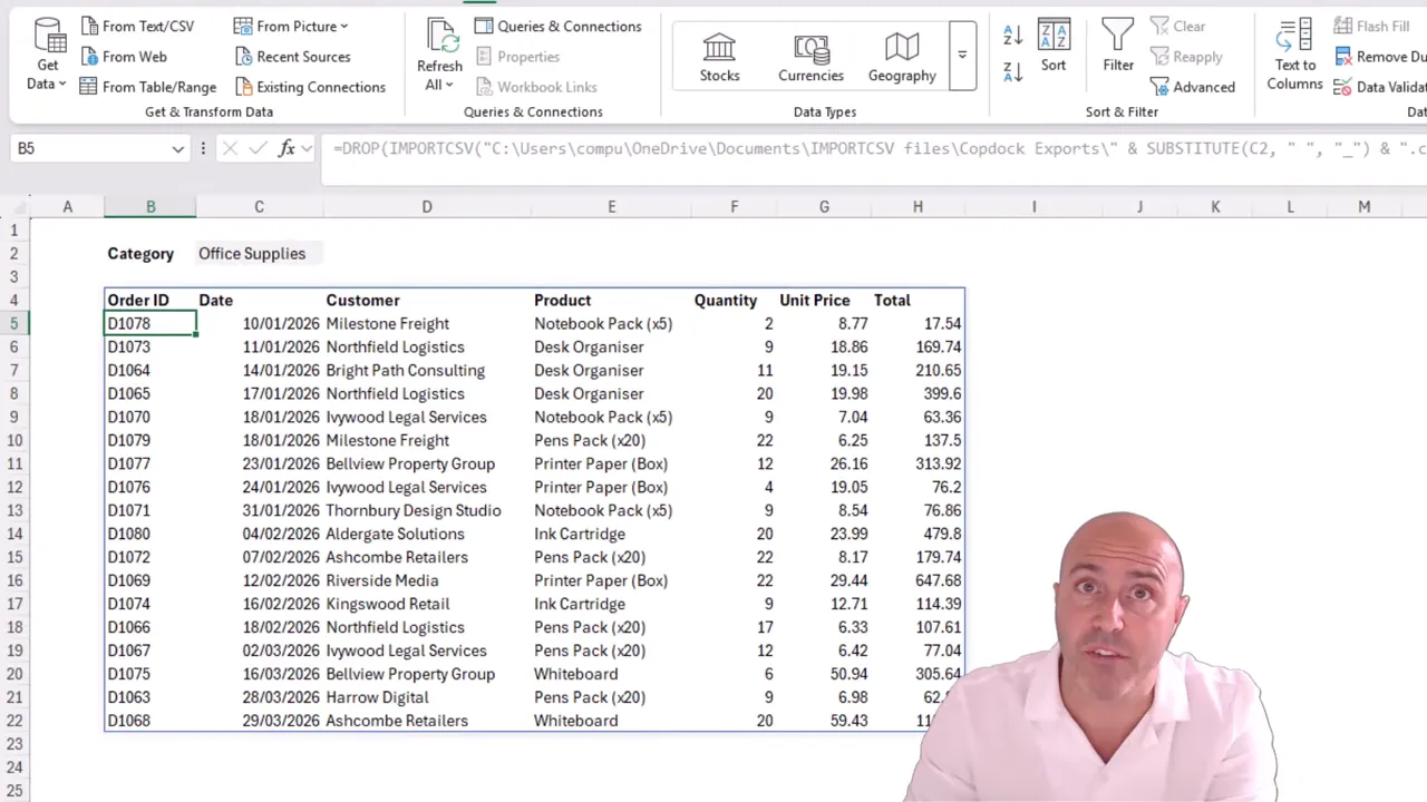
We now have a single formula that chooses the CSV from the drop-down, adjusts the category text to match the filename, imports the data, and removes the unnecessary final column. A nice, compact solution.
Fix Date Conflicts with the Source Locale
For the final example, we will import a CSV containing US vendor invoices.
My regional settings are UK, where dates use a day, month, year structure. The source uses US month, day, year dates. A basic import brings in the records, but the dates are not all interpreted correctly.
This is a job for the locale argument within IMPORTCSV:
- Edit the IMPORTCSV formula.
- Leave the optional arguments you do not need empty, using commas to move to the locale argument.
- Choose English (United States) from Excel's locale suggestions.
- Complete the formula and press Enter.
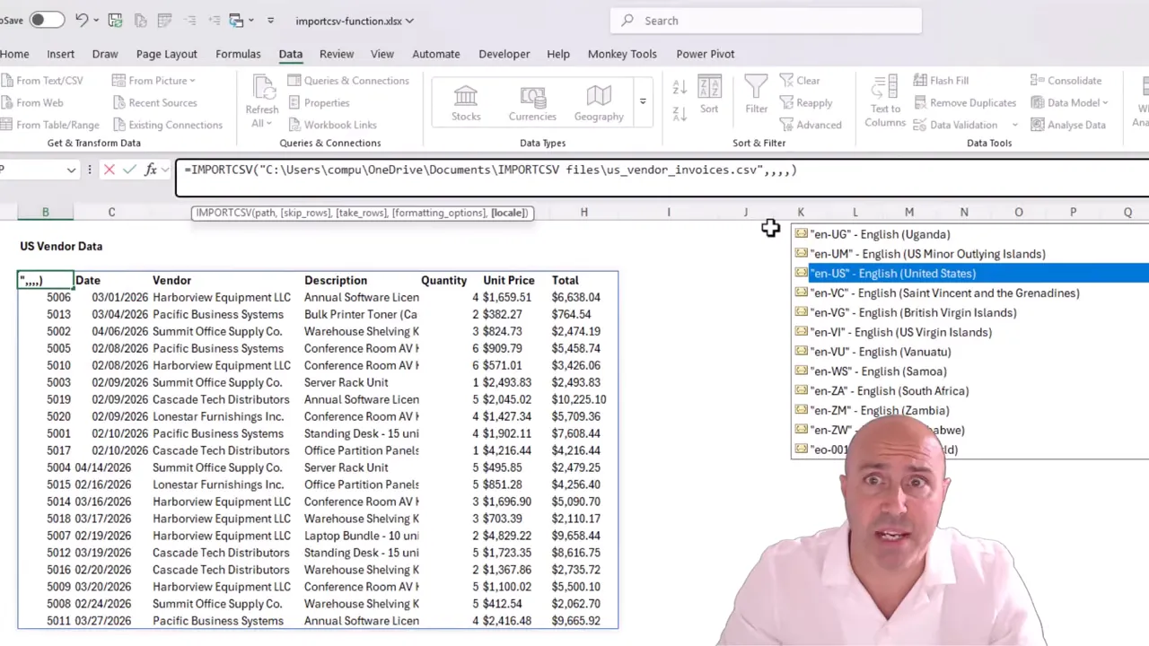
The dates are now interpreted correctly and displayed in the workbook's day, month, year structure.
The important point is to specify where the source data comes from, rather than simply choosing the region you want the output to resemble. Excel needs to understand the incoming values first. The same option is useful when working with regional number conventions, such as different decimal separators.
When to Use IMPORTCSV Instead of Power Query
IMPORTCSV makes a great alternative when the task is straightforward and a worksheet formula is a natural fit.
- Use IMPORTCSV for a lightweight CSV import, a refreshable spilled result, or a source file selected dynamically through worksheet cells.
- Use Power Query when data connections and transformations are the main task, especially when the preparation process is more involved.
Microsoft's Power Query overview explains its broader role in connecting to and preparing data. For a more involved file-combination example, see my tutorial on combining files with different headers using Power Query.
The two tools have different strengths. IMPORTCSV is not a replacement for Power Query, but it makes importing CSVs wonderfully simple. Combine it with other Excel functions, and that single import formula can become a creative, dynamic solution.


