Slicers are excellent filtering tools in Excel, but there is much more to them than clicking a button to filter a PivotTable. A few simple settings can make them more compact, easier to use, and better suited to a dashboard. Add a helper column and some formulas, and they can control formula-driven reports too.
These seven Excel slicer tips cover both sides: straightforward layout improvements and more advanced formula techniques. There is also a bonus tip for sorting slicer buttons into a sensible order rather than accepting alphabetical order.
You can follow along with the practice workbook.
Table of Contents
- 1. Use Icons or Emojis in Your Slicers
- 2. Switch a Slicer to a Horizontal Layout
- 3. Use Excel Slicers with Worksheet Formulas
- 4. Display the Selected Slicer Values in a Chart Title
- 5. Hide Slicer Items with No Data
- 6. Filter Multiple PivotTables with One Slicer
- 7. Stop Slicers Moving When a PivotTable Updates
- Bonus Tip: Sort Slicer Buttons with a Custom List
1. Use Icons or Emojis in Your Slicers
Text labels are perfectly useful, but they can take up quite a bit of space. Long category names require wide buttons, which means a larger slicer. Where a category has an obvious visual equivalent, an emoji can provide a compact alternative.
The important point is that the icons come from a column in the source data. We are not placing pictures over the slicer buttons. Excel uses the emoji values as the items to filter.
- Add a column to the source table named Category Icon.
- Enter an appropriate emoji for each category, using the same emoji for every row belonging to that category.
- On Windows, press Windows + period to open the emoji picker, then search for the icon you want.
- Remove the existing category slicer if you are replacing it.
- Select the PivotTable, then choose PivotTable Analyze > Insert Slicer.
- Select Category Icon and click OK.
For example, a burger icon can represent food. The resulting slicer filters the PivotTable just as a text-based category slicer would, but its buttons need much less room.
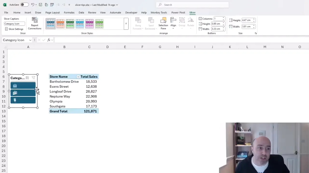
Resize the slicer and choose a suitable style from the Slicer tab. A narrow vertical slicer can sit neatly beside the report instead of taking up a large section of the worksheet.
2. Switch a Slicer to a Horizontal Layout
A slicer does not have to be a vertical list. If you only have a few options, a horizontal layout often fits much more naturally above a report.
The setting you need is Columns on the Slicer tab.
- Select the slicer.
- Open the Slicer tab on the ribbon.
- Change Columns to the number of items you want across the slicer.
- Adjust the slicer's width and height to suit the new arrangement.
In the example, there are three category icons. Setting Columns to 3 places all three buttons on a single row. The slicer can then sit above the PivotTable at roughly the same width as the report.
This is a particularly nice alternative when there are only a handful of choices. Instead of leaving space down the side of the worksheet, you can use a compact strip of filter buttons across the top.
3. Use Excel Slicers with Worksheet Formulas
Slicers are not limited to PivotTables. They can also filter an Excel table. The challenge is getting worksheet formulas to respect the rows that the slicer has filtered out.
Suppose a report uses GROUPBY to calculate sums and counts from a sales table. A slicer connected to that table may successfully hide all categories except Beverages, while the formula report continues to show results for the full data set.
The slicer is working. The formula simply needs a way to identify which source rows remain visible.
Create a visibility helper column
In the source table, add a column named Filter. Use the following formula to count the numeric Order ID in the current row while ignoring hidden rows:
=AGGREGATE(2,5,[@[Order ID]])There are three parts to understand:
- 2 tells AGGREGATE to use COUNT.
- 5 tells it to ignore hidden rows, allowing the calculation to respond to the slicer's filtering.
- [@[Order ID]] refers to the Order ID in this row, not the entire Order ID column.
Because the example uses numeric Order IDs, a visible row returns 1. A row excluded by the filter returns 0.
That numeric detail matters. COUNT counts numbers, so use a populated numeric field for this technique. Microsoft’s AGGREGATE function reference explains the function numbers and available options.
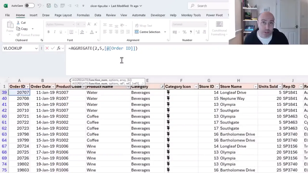
You cannot see the zeros while those rows are filtered out, of course. One useful check is to select the Filter column and compare Count with Sum on the status bar. In this example, after allowing for the header counted by Count, they match for the visible rows because those rows all contain ones.
Add the visibility condition to your report formula
Once the helper column exists, the condition for including a row is straightforward:
tblSales[Filter]=1Here, tblSales is the source table's name. In the GROUPBY formula, enter this condition in the filter_array argument. Keep the existing grouping fields, values, and calculations, but include only rows where Filter equals 1.
Now, when you select a category in the slicer, the table is filtered, the helper column identifies the visible records, and GROUPBY uses only those records.
The same idea works with other functions:
- Use Filter equals 1 as an additional criterion in SUMIFS.
- Add the same criterion to COUNTIFS.
- Use tblSales[Filter]=1 as the include condition in FILTER.
That helper column is the connection between the slicer and the formulas. Once it is in place, you can build formula-driven reports without having to use a PivotTable for every calculation.
4. Display the Selected Slicer Values in a Chart Title
A chart title such as “Sales for Beverages” is much more informative than a fixed title that gives no indication of the current filter.
This becomes especially useful in a larger dashboard, where several slicers may affect the results and the active combination is not immediately obvious.
We can reuse the Filter helper column from the previous tip to create a label listing the categories represented by the visible rows.
Build the title in a worksheet cell
The formula combines four functions:
- FILTER returns category names from rows where the Filter column equals 1.
- UNIQUE removes duplicate category names.
- SORT arranges those names alphabetically.
- TEXTJOIN combines them into a comma-separated list.
Using the sales table and Category column, the formula is:
="Sales for "&TEXTJOIN(", ",TRUE,SORT(UNIQUE(FILTER(tblSales[Category],tblSales[Filter]=1))))It looks like quite a formula at first, but break it into those four jobs and it is not nearly as scary.
Select Beverages and the label lists Beverages. Hold Ctrl and select Food as well, and both categories appear. Clear the slicer filter, and the label lists all categories represented in the visible data.
Link the chart title to the formula cell
- Enter the title formula in a worksheet cell, such as C7.
- Select the chart title.
- Click in the formula bar and enter a reference to that cell, including the worksheet name.
- Press Enter.
The chart title now displays the cell's result and updates as the slicer selection changes.
This technique is not limited to chart titles. The same text could be used as a report label or another dashboard annotation. More precisely, it describes the categories remaining in the filtered source data, which makes it useful when several filters are working together.
5. Hide Slicer Items with No Data
Dependent slicers are a good example of how a small settings change can make a report easier to use.
Imagine two slicers: one for Category and one for Product Name. Select Food in the category slicer, and the product slicer prioritizes the food products. Products with no data under that selection may still appear underneath, but with a different visual treatment.
That can be useful, but sometimes you would rather remove the irrelevant choices entirely.
- Right-click the dependent slicer, in this case Product Name.
- Select Slicer Settings.
- Check Hide items with no data.
- Click OK.
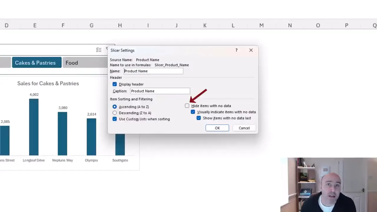
Now, selecting Food presents only the products with data for Food. Selecting Cakes & Pastries changes the available product list accordingly.
The distinction is simple: visually indicating items with no data leaves them in the slicer; hiding them removes them from the displayed list. Choose the behavior that makes the most sense for your report.
6. Filter Multiple PivotTables with One Slicer
One of the biggest advantages of slicers is the ability to filter several reports from a single control, including reports on different worksheets.
For example, one category slicer can update a store sales PivotTable and a chart showing a different breakdown of the same data.
The setting that controls this is Report Connections.
- Select the slicer.
- Open the Slicer tab.
- Click Report Connections.
- Check each available PivotTable that the slicer should control.
- Click OK.
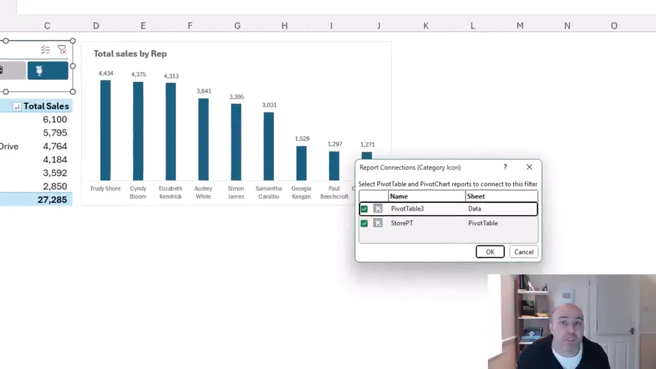
The dialog lists the PivotTables and their worksheets, so the reports do not need to be on the same sheet.
Give your PivotTables meaningful names. With two reports, a default name such as PivotTable3 is manageable. With a larger dashboard, names such as StorePT make it much easier to choose the correct connections.
There is also a small but useful distinction with PivotCharts: the slicer connects to the chart's underlying PivotTable rather than directly to the chart itself. Filtering that PivotTable updates the PivotChart.
If you uncheck StorePT, for example, the slicer stops affecting that PivotTable. A chart based on another connected PivotTable can continue to respond. Recheck StorePT and both reports are controlled again.
You can achieve the same single-filter behavior with formula-driven reports. Each report simply needs to use the visibility condition from tip three against the same slicer-filtered source table.
7. Stop Slicers Moving When a PivotTable Updates
Have you ever clicked a slicer button and found that the slicer itself shifted position?
In this example, selecting a different course level changes the course names displayed in a PivotTable. Excel adjusts the width of column A to fit those names, and the slicer moves because its position is tied to the cells.
There are two settings worth knowing: one for the slicer and one for the PivotTable.
Keep the slicer in a fixed position
- Right-click the slicer.
- Select Size and Properties.
- Expand Properties in the formatting pane.
- Select Don't move or size with cells.
The slicer in this example was set to move with cells without resizing. Changing it to Don't move or size with cells keeps it in place when column widths change.
Stop the PivotTable from changing column widths
For this particular report, I would also consider stopping the automatic width adjustment at its source.
- Select a slicer item that displays the longest course names, so you can establish a suitable column width.
- Right-click the PivotTable and select PivotTable Options.
- On Layout & Format, clear Autofit column widths on update.
- Click OK.
Now the PivotTable no longer changes the column widths as you filter between levels.
You do not necessarily need both changes. In this example, the PivotTable's automatic column resizing was the cause of the movement, so disabling that alone addresses it. Knowing both settings gives you control over the report layout and the slicer's behavior.
Bonus Tip: Sort Slicer Buttons with a Custom List
Alphabetical order is not always the right order.
For course levels, Beginners, Intermediate, Advanced is much more sensible than Advanced, Beginners, Intermediate. A custom list lets Excel use that logical sequence.
- Go to File > Options > Advanced.
- Scroll down to the General section and click Edit Custom Lists.
- Create a list containing Beginners, Intermediate, and Advanced in that order, using one entry per line.
- Add the list and confirm the dialogs.
- Right-click the slicer and open Slicer Settings.
- Make sure Use Custom Lists when sorting is checked.
That setting is normally enabled, but it is worth checking if your slicer is still using alphabetical order.
With the custom list in place, the buttons follow the progression of the course levels rather than the alphabet. It is a small finishing touch, but it makes the slicer much more natural to use.
Between compact layouts, formula-aware filtering, clear labels, shared report connections, and stable positioning, slicers can do far more than filter a single PivotTable. The most useful improvements are often just one setting or one helper column away.


