Beautiful, interactive dashboards do not belong exclusively to Power BI or Tableau. Excel is a blank canvas too. The difference is often not the software, but how we combine the tools we already have.
Two things make Power BI dashboards particularly appealing: interactivity and design. We can bring a surprising amount of both into Excel using slicers, charts, formulas, shapes, linked text boxes and pictures. The main techniques here need no VBA or add-ins.
There is an important distinction, though. Clicking a chart point in Power BI can filter the rest of a report automatically. These Excel examples use explicit controls, such as slicers, dropdowns and checkboxes, rather than reproducing that entire interaction model.
Our example data comes from Santa’s business: reindeers, carrots, sleeping hours and gift deliveries. It is a little more fun than another sales report, but the techniques transfer directly to business dashboards. You can explore the finished examples in the downloadable Excel workbooks.
What You'll Learn
- Plan dashboard content, refreshes and layout around the people who will use it.
- Combine slicers and helper series to create dynamic highlights without losing comparison context.
- Build polished KPI cards from linked text boxes, shapes, pictures and small charts.
- Use internal hyperlinks and hidden sheet tabs for navigation and light or dark dashboard designs.
Table of Contents
- Start With the User, Not the Charts
- Build a Design System You Can Reuse
- Create the Interactive Foundation With PivotTables and Slicers
- Use Helper Series to Make Charts Tell a Story
- Use a Slicer to Highlight Instead of Filter
- Build Power BI-Style KPI Cards From Simple Objects
- Put Dropdowns Inside a Polished KPI Design
- Add Dashboard Navigation Without VBA
- Hide the Spreadsheet Interface, Not the Destination Sheets
- Create a Light and Dark Dashboard Switch
- Make the Finished Workbook Practical to Use
- The Real Skill Is Combining Familiar Tools
Start With the User, Not the Charts
A dashboard can look wonderful to its developer and still be confusing to everyone else. You know the data, the calculations and the reasons behind each chart. Your users may not.
Before opening the chart menu, answer a few questions:
- Who is the end user? How familiar are they with the data?
- What is the purpose? Are they identifying patterns, tracking performance or checking a few key indicators?
- How will data arrive? What needs to happen when new information becomes available?
- Which controls make sense? Do users need to filter by date, category or another field?
- What do they actually need? A dashboard is not always better than a simple PivotTable.
I really recommend spending time getting to know the data before designing anything. Explore the columns, check whether you have dates or times, and understand how the dataset is structured. That work helps you choose useful charts and sensible slicers.
Also think about refreshes from the beginning. I use Power Query to bring data in from other sources, aiming for a process where the user can refresh the data and the supporting PivotTables without manually copying information between programs.
Finally, sketch the dashboard and discuss it with the user. A rough layout is enough to check that you are solving the right problem. Finding out that someone only wanted a PivotTable is much less painful before you have finished a beautifully formatted dashboard!
Build a Design System You Can Reuse
Keep an inspiration collection
When I first started creating dashboards, I could spend hours on the design and still not feel happy with the result. Building an inspiration collection made the process much easier.
Whenever you find something you like, save it. It might be a complete dashboard, but it could also be a colour combination, a chart, a navigation panel or a single KPI card.
The useful part is asking what exactly you like about it. Is it the layout? The spacing? The way a change indicator is displayed? You can then combine those ideas into a new design rather than starting from nothing every time.
You do not need to be a graphic designer to choose a good palette. A colour palette tester with a sample dashboard helps you see how colours work together before applying them throughout a workbook. Dashboard inspiration boards, including the Pinterest collection by Mara Pereira, are also useful starting points. The example workbooks include design resources to explore.
Use a clear visual hierarchy
A reliable starting layout is:
- KPI cards across the top for the most important numbers.
- Navigation or slicers on the left for moving around and filtering.
- Charts in the middle for comparisons, trends and supporting detail.
The logic is simple. Someone with very little time should be able to understand the headline numbers quickly, then move into the charts when they need more information.
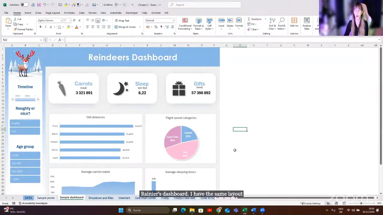
Once you have a layout that works, turn it into a reusable template. Reusing a good foundation is much more efficient than redesigning every report.
Pay attention to the small details
The difference between a basic KPI and a polished one often comes down to small choices: a relevant icon, a currency symbol, stronger number formatting, a shadow or a clear positive and negative indicator.
For a revenue card, a money icon and a euro symbol immediately establish the subject and unit. Colour can help communicate a change, while carefully chosen shadows and gradients can give the card a more modern appearance.
Use a short design check before finishing: Is the palette consistent? Are the important numbers easy to identify? Do icons and visual indicators help explain the data? These details should make the dashboard easier to understand, not simply more decorative.
Create the Interactive Foundation With PivotTables and Slicers
If you are new to dashboards, PivotTables are an excellent place to start. Dynamic array formulas give us other options, but we do not have to begin with the most advanced approach.
The basic structure of the reindeer dashboard is:
- Store the source data in an Excel table.
- Create PivotTables for the measures and comparisons you need.
- Create PivotCharts from those PivotTables.
- Create small summary PivotTables for individual KPI values.
- Place the charts and KPI objects on a dedicated dashboard worksheet.
- Add slicers and connect them to the relevant PivotTables.
The small summary PivotTables are especially useful. One might calculate total gift deliveries, while another returns the sleeping-hours figure required for a KPI card.
Connect each slicer to the whole dashboard
A new slicer is initially connected to the PivotTable from which you created it. It does not automatically control every chart on the page.
Select the slicer, open Slicer > Report Connections, and tick each relevant PivotTable. Include the summary PivotTables that feed your KPI cards, not just those behind the charts.
Give your PivotTables meaningful names first. A name such as RD_Carrots is much easier to recognise in the connections list than a series of default names.
Link text boxes to KPI cells
A dynamic KPI number does not need to be typed into a shape manually:
- Insert a text box.
- Select the text box itself, rather than editing its text.
- Click the formula bar and type
=. - Select the cell containing the required result and press Enter.
The text box now displays the cell value. If that cell belongs to a summary PivotTable connected to your slicer, the KPI updates with the rest of the dashboard.
That is the essential connection: slicer to PivotTable, PivotTable result to text box. Much of the remaining work is formatting.
Use Helper Series to Make Charts Tell a Story
One of the most useful chart techniques is to stop thinking of the finished visual as one object. Instead, break it into pieces.
Many of these examples have two layers: a neutral background containing the full dataset and a coloured foreground containing only the information we want to emphasise. Depending on the example, these can be series within one chart or separate charts positioned together.
Highlight the maximum value dynamically
Suppose a dropdown selects a reindeer and the chart shows how many carrots that reindeer eats at each meal. Rudolph eats most of his carrots at dinner, while Cupid eats most at second breakfast. We want the highest column to change colour automatically.
The calculation has three parts:
- Use XLOOKUP to retrieve the selected reindeer’s meal values.
- Use MAX to find the largest value in those results.
- Create a helper row that returns the value when it equals the maximum, and NA() otherwise.
The helper logic is =IF(value=MAX(selected_values),value,NA()), where the descriptive names represent your own cell references or ranges.
The base series displays all meals in grey. The helper series supplies the coloured highlight. In this column-chart example, the #N/A results leave the unwanted columns unplotted, so only the maximum appears in the highlight colour.
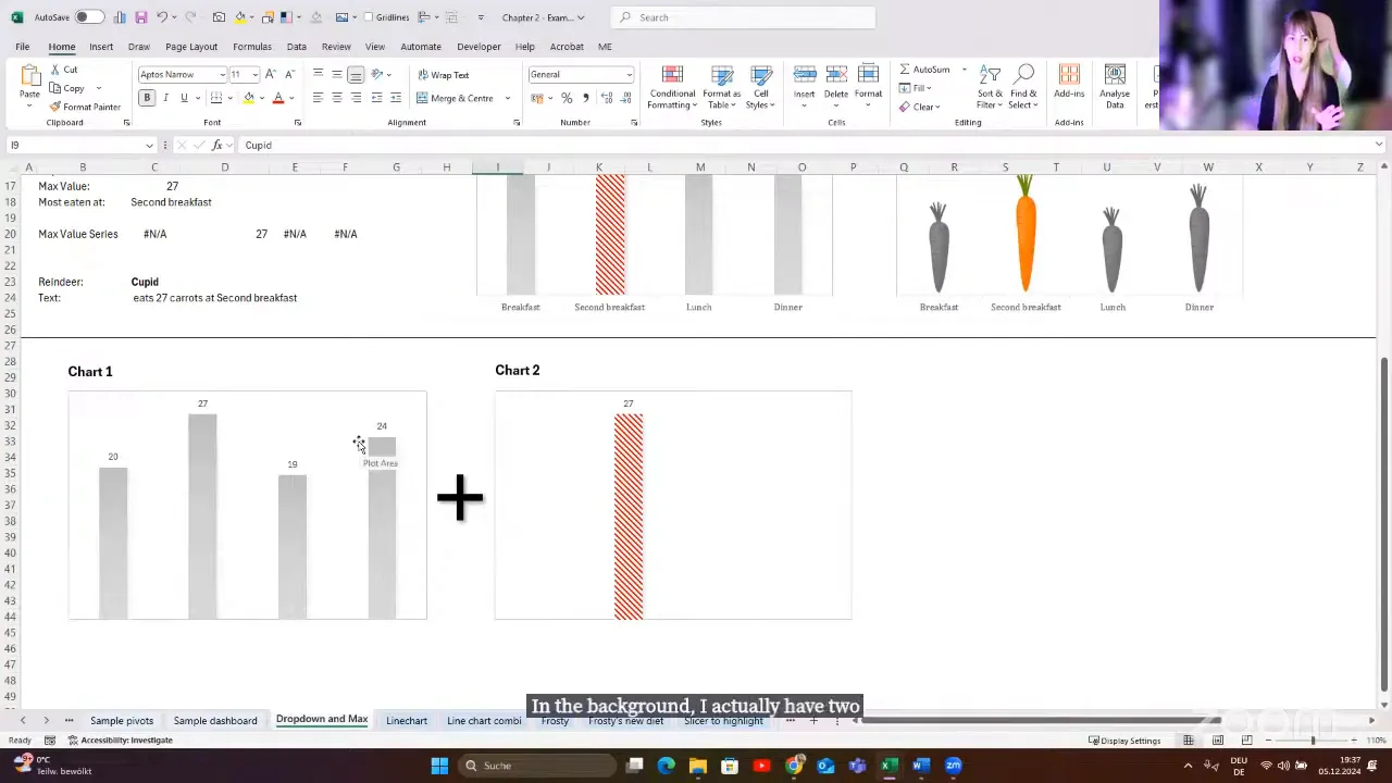
A quick way to add helper data is to copy the helper range, select the existing chart and paste. Format the added series and position it to overlap the base columns.
The same idea can be more playful too. In the carrot-consumption example, pictures of carrots replace ordinary columns. The calculation behind the highlight is still the same.
Highlight a selected date interval
For a line chart, keep the complete trend in grey and add a second line in red. The helper series returns the original value only when its date falls within the selected interval. Outside that interval, it returns NA().
Now the selected period stands out without removing the surrounding history. It is a simple way to direct attention while keeping context.
Highlight one line without hiding the others
A slicer can also work with a normal Excel table rather than a PivotTable. The challenge is turning the filtered table into a selection that other formulas can use.
In the example, SUBTOTAL retrieves a numeric identifier from the visible rows. With a single reindeer selected, that identifier can drive an XLOOKUP or an INDIRECT-based helper range.
The resulting helper series is drawn in red above the other reindeers’ lines. A label identifies the highlighted reindeer, so the user does not have to work it out from colour alone. Microsoft’s SUBTOTAL documentation explains its behaviour with filtered rows.
Show or hide chart commentary with a checkbox
Sometimes a line chart shows what happened, but not why. Comments can explain important events, such as Frosty’s injury or the discovery of a magic carrot in our example data.
Store those comments in a helper column and use a checkbox to control whether they appear. A second series supplies the relevant event points, with labels connected to the prepared commentary.
When the checkbox is enabled, the annotations explain the story. When it is disabled, the chart returns to a cleaner view. This gives the user control over how much explanation is visible.
Make a pie-chart selection stand out
Pie charts become difficult to read when they contain too many categories, especially when someone needs to compare similarly sized slices. But sometimes a user specifically wants one. We can still make the selected category easier to identify.
This example uses two aligned pie charts:
- The lower chart contains every category, formatted in grey.
- The upper chart contains three calculated portions: everything before the selection, the selected category, and everything after it.
The selected portion receives the highlight colour. The other portions of the upper chart leave the lower chart visible. Because the totals and order match, the highlighted slice sits in the correct position.
Again, the useful question is not “How do I make this complicated chart?” It is “Which simple pieces do I need?”
Use a Slicer to Highlight Instead of Filter
Filtering and highlighting answer different questions. If selecting one reindeer removes all the others, it becomes difficult to compare their performance.
To preserve that comparison, keep an unfiltered base dataset for the grey chart. Use a separate slicer-connected table to determine the selection, then create a helper series that returns:
- The original value for the selected reindeer.
- Zero for the other reindeers in this bar-chart example.
The coloured helper series sits over the grey base series. The selection changes, but the other reindeers remain visible.
The important distinction is that the slicer controls the highlight calculation, not the full comparison dataset. Dynamic arrays can help prepare the chart data, while SUBTOTAL supplies the visible selection from the filtered table.
Add a picture that changes with the selection
Picture in Cell is one of my favourite Excel features for this kind of dashboard. Store an image beside each reindeer’s data, then use XLOOKUP to return the matching picture.
The workflow is:
- Insert each picture into a cell alongside its matching record.
- Use XLOOKUP to return the picture for the selected reindeer.
- Create a reference to that result picture and position it on the dashboard.
Now the image updates with the slicer selection. The same underlying idea also works for the playful dropdown example that switches between Saint Nicholas and Krampus: a small control can change the visual experience as well as the numbers.
Build Power BI-Style KPI Cards From Simple Objects
A KPI card may look like a special visual, but in Excel it can be a group of familiar objects:
- A rounded rectangle for the background.
- A linked text box for the main number.
- A linked text box for the selected name or category.
- Static labels and an appropriate icon.
- A dynamic change indicator.
- Optionally, a small chart showing the trend.
Build the pieces, format them, then group them together. That is the basic technique.
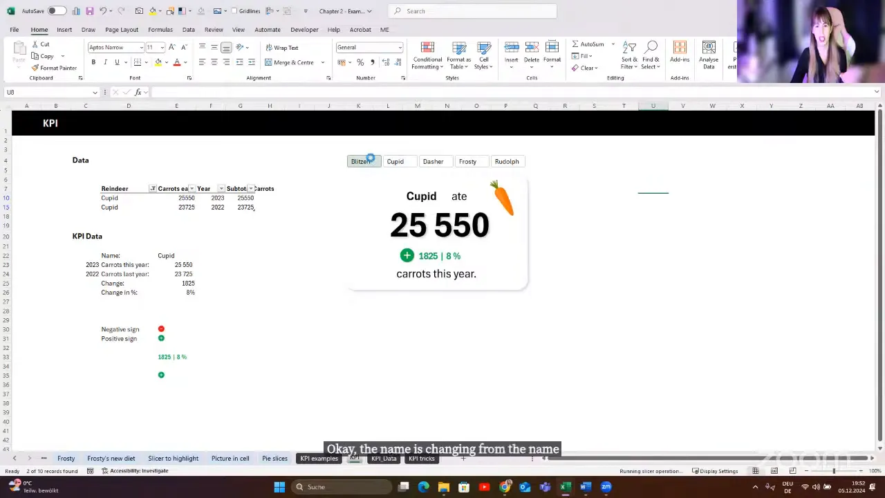
Switch positive and negative icons
For a dynamic status icon, prepare separate positive and negative images. I created the signs in Canva, placed them in cells and used an IF formula to return the appropriate image based on the change from the previous year.
Create a reference to the result picture, place it on the card, and group it with the other objects. The same approach can switch between red and green rounded backgrounds behind a change indicator, or even behind the entire card.
Preserve conditional formatting with the Camera tool
A text box linked to a cell is useful for displaying its value, but it is not the same as reproducing all of that cell’s conditional formatting.
For dynamically coloured change text, conditionally format the source cell and use Excel’s Camera tool to create a live picture of it. Place that picture on the KPI card.
Check the picture formatting carefully. A default white background or border can make the result look pasted on. Adjust those settings so it blends with the card.
This is a dynamic linked picture, not a static screenshot. When the source cell changes, its displayed result changes too.
Create a colour-changing accent bar with a chart
A thin red, green or grey line can make a card feel much more polished. It can also be an ordinary chart.
Create three helper values:
- Negative: 100 when the change is negative, otherwise zero.
- Positive: 100 when the change is positive, otherwise zero.
- Neutral: 100 when the change is zero, otherwise zero.
Use these values in a small bar chart and format the three series red, green and grey. Remove the chart elements you do not need, then resize it into a narrow accent. Only the relevant colour remains visible.
Add trend context
A headline number becomes more useful when it also shows direction over time. One of the example cards combines a large value, a change indicator and a small line chart.
There is no special KPI machinery behind it. It is simply another chart placed alongside linked text boxes and a dynamic picture. Breaking the design into pieces makes it much less intimidating.
Put Dropdowns Inside a Polished KPI Design
A KPI can become more useful when the user can choose its metric or comparison period. For example, a selection might switch between carrots, sleep and gifts, or between last month, the last six months and last year.
A combo box linked to a cell can drive the required lookup formulas. The difficulty is appearance: the traditional control offers limited design flexibility.
A different approach is to use a dropdown directly in a worksheet cell, then build the card around it.
Leave a cutout in the card background
A normal rectangle placed over a cell blocks access to that cell. To keep the dropdown usable, create a card background with an opening where the cell needs to remain visible.
- Create the card background in PowerPoint.
- Create another shape over the area intended for the dropdown.
- Use the shape subtraction feature to cut that area out.
- Bring the resulting background into Excel.
- Align the opening with the dropdown cell.
- Position the linked values and other card elements around it.
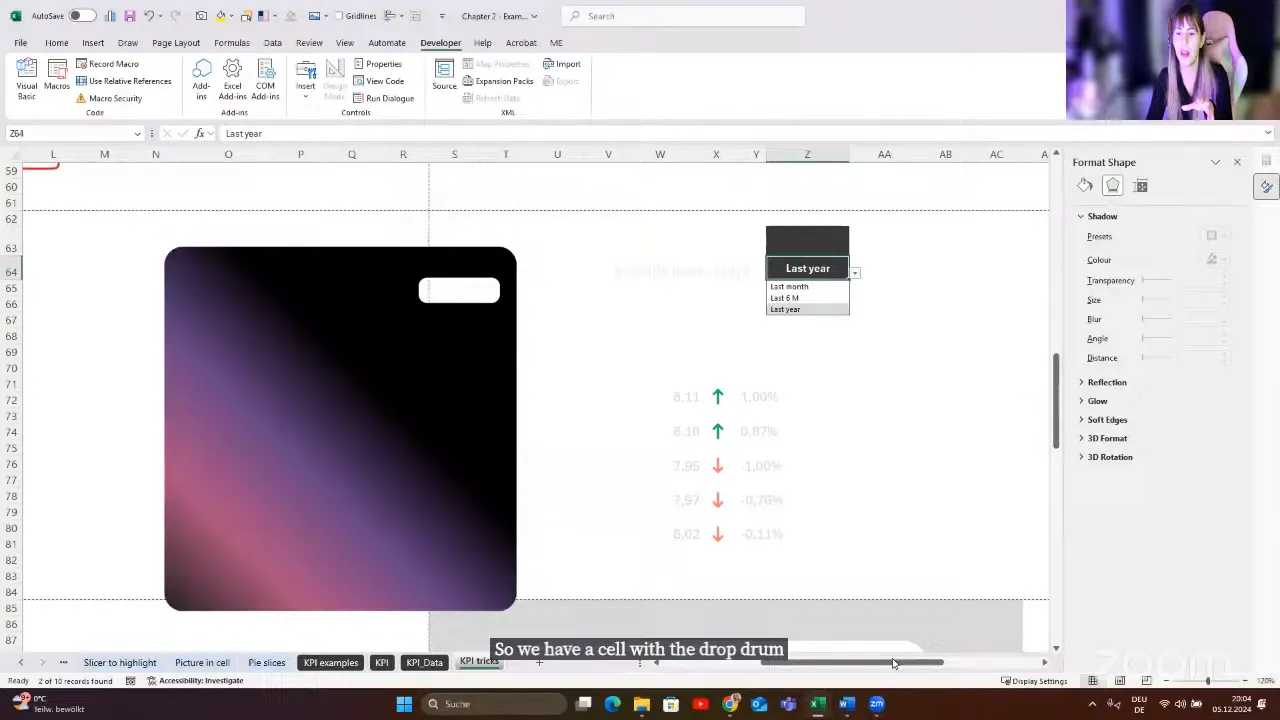
It is a workaround, certainly, but it lets a normal cell control sit inside a much more polished design. The same idea can expose a heat map, a range of cells or other worksheet content without giving up the surrounding background.
Add Dashboard Navigation Without VBA
A Power BI-style navigation panel can be built with shapes and ordinary internal links. You do not need a macro just to move between worksheets.
For the reindeer example, create separate dashboard pages for sleeping hours, carrot consumption and gift deliveries. Keep their layouts consistent so moving between them feels natural.
- Build the first page with its navigation shapes.
- Duplicate it for the other metrics.
- Update each page’s data links, charts and labels.
- Right-click a navigation shape and select Link.
- Choose Place in This Document and select the destination worksheet and cell.
- Format the current page’s navigation item differently from the others.
You can use a left-side menu, or create a compact carousel-style design with left and right arrows and small page indicators. Both use the same linking technique.
In the compact example, the current page indicator is white and the others are more transparent. That tiny detail helps the user understand where they are.
I prefer to keep supporting data on separate worksheets where practical. It makes it easier to keep the dashboard pages focused on the interface rather than the calculations.
Hide the Spreadsheet Interface, Not the Destination Sheets
Once navigation is working, a few display changes can make the workbook feel much less like a worksheet.
- Under View, turn off gridlines.
- Hide the formula bar when it is not needed.
- Hide row and column headings.
- Double-click a ribbon tab to collapse the ribbon.
- Hide worksheet tabs through the workbook display settings.
The last point needs care. Hiding a worksheet is not the same as hiding its tab display. An ordinary hyperlink cannot navigate to a hidden destination worksheet.
In desktop Excel for Windows, go to File > Options > Advanced > Display options for this workbook, then clear Show sheet tabs.
This removes the tab strip while leaving the destination sheets available to your navigation links. Build and test the navigation first, then change the display setting.
Create a Light and Dark Dashboard Switch
A light and dark dashboard switch uses exactly the same navigation trick. It does not need to change every shape and chart dynamically.
- Create the dashboard in one colour scheme.
- Duplicate the worksheet.
- Reformat the duplicate with the alternative background, text and chart colours.
- Add Light and Dark navigation buttons.
- Link each button to the appropriate worksheet.
- Hide the sheet-tab display for a cleaner experience.
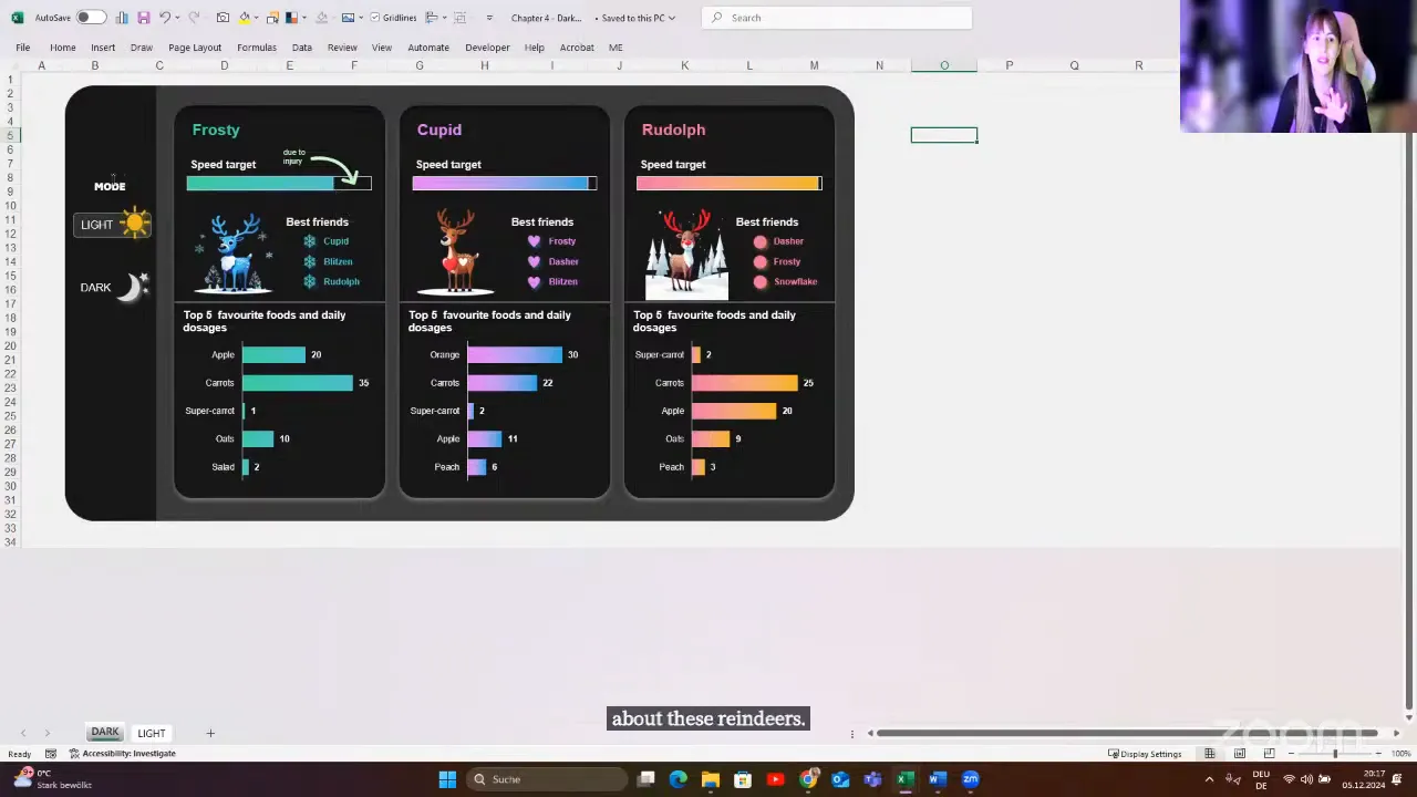
Clicking Light or Dark moves to the corresponding version. To the user, it feels like a theme switch. Underneath, it is simply two consistently designed pages connected with links.
This is a dashboard design technique, not a change to Excel’s application theme. Its strength is its simplicity.
Make the Finished Workbook Practical to Use
Choose techniques for the Excel version
These examples were built in Microsoft 365. Features such as dynamic arrays and Picture in Cell may require another approach in older Excel versions.
That does not mean the whole design is impossible. It means checking which part needs a workaround. Build for the version your users actually have.
I also prefer desktop Excel for advanced dashboard work. Excel for the web has a different interface and a different experience, so do not assume every desktop technique will transfer unchanged.
Keep sparklines in cells when that helps the user
Sparklines can work beautifully in a dashboard without being converted into pictures. Leave them in their worksheet cells and format the surrounding area to match the dashboard.
There are two useful reasons to do this:
- Camera pictures can lose visual quality when enlarged.
- A picture does not let the user select and copy the underlying cell values.
If your design uses background shapes, either leave the cell area uncovered or use the cutout technique. A later reindeer example used VBA for click-based selection, but the sparkline layout itself does not require that interaction.
Design the handover for the client’s skill level
A client dashboard should be easy to use and reasonably easy to maintain. For less experienced users, I keep supporting data out of the way and protect relevant worksheets so the intended interaction is through slicers and controls.
For more advanced users, clear Excel tables, meaningful names and understandable formulas make changes easier. I do not automatically use LAMBDA or the most sophisticated formula available if the person maintaining the workbook will struggle with it.
The right solution depends on the client. A clever workbook that nobody can maintain is not necessarily a good workbook.
Keep the fundamentals, even when using AI
AI can be a useful helper, but it does not remove the need to understand your data and check the result. Structure, data types, tables and ranges still matter.
Knowing the steps for a feature is only part of the skill. You also need to recognise when it does not work, why the result is wrong and which alternative makes sense. That applies to AI-generated formulas just as much as it applies to a quick Flash Fill trick.
The Real Skill Is Combining Familiar Tools
Most of these techniques use tools you may already know: XLOOKUP, IF, charts, slicers, shapes and links. The interesting part is how they work together.
A helper series turns a plain chart into a guided comparison. A linked text box turns a summary cell into a KPI. A picture formula supplies a changing status icon. A few shapes and hyperlinks turn worksheets into dashboard pages.
You do not need to rebuild everything at once. Start with one clear improvement, perhaps a dynamically highlighted maximum or a properly connected slicer. Then build your own collection of reusable pieces.
With a little creativity and attention to detail, Excel can feel much less like a spreadsheet and much more like a thoughtfully designed application.


